1. Crash Pulse Reconstruction from Accelero
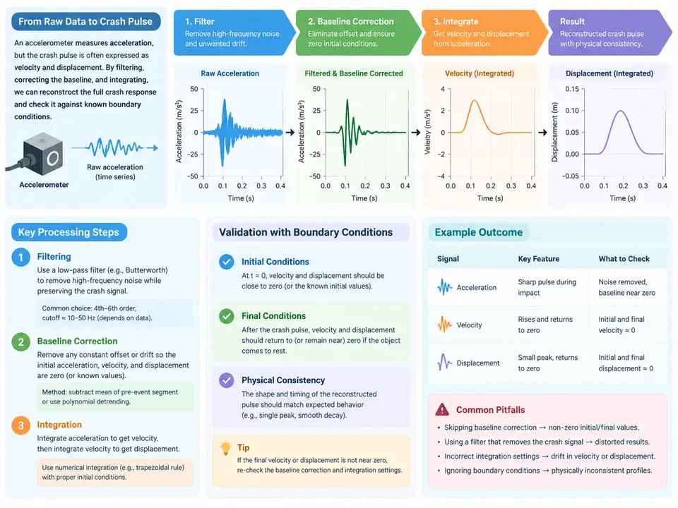
Why Raw Accelerometer Data Cannot Be Integrated Directly
A crash pulse is the acceleration–time history measured on a vehicle body or sled during an impact. From it we derive two quantities that matter for occupant restraint design: the velocity change Δv (integral of acceleration) and the displacement (double integral). The raw signal from a piezoelectric or piezoresistive accelerometer, however, is never ready for integration. Three defects dominate:
- DC offset / baseline drift. A constant bias of even 0.05 g integrated over 100 ms produces a spurious 0.049 m/s velocity error, and double integration turns that into a large, physically impossible displacement ramp.
- High-frequency noise. Sensor resonance, mounting ringing, and electrical noise integrate into velocity noise that grows with time; unfiltered, the displacement curve diverges.
- Integration drift. Any residual bias after correction still accumulates quadratically in displacement, so boundary conditions must be enforced explicitly.
The reconstruction workflow therefore is: baseline correction → low-pass filtering → integration to velocity → integration to displacement → boundary-condition validation. The order matters: correcting the baseline before filtering avoids feeding a step into the filter's transient, and filtering before integration suppresses noise amplification.
Reference Conventions Used in This Case
All signals follow the SAE J211 / ISO 6487 sign convention for a frontal impact: positive acceleration points forward (the direction the vehicle travels before impact). During a frontal crash the vehicle decelerates, so the measured longitudinal acceleration is negative. Velocity is the integral of acceleration, so Δv is negative (the vehicle slows). Displacement is measured along the same axis; a negative displacement means the body moved forward relative to its initial position. Keep this convention consistent across the data, the code, and the SVG below.
Worked Example: Reconstructing a 50 km/h Frontal Pulse
Assume a 100 ms sampled record at 10 kHz (1001 samples, t = 0…0.100 s) from a body-mounted accelerometer. The teaching dataset below is synthetic but shaped like a real frontal pulse: a short rise, a plateau near −30 g, and a decay back toward zero, with a deliberate +0.08 g bias and 2 g RMS broadband noise added to simulate a realistic raw channel.
import numpy as np
from scipy.signal import butter, filtfilt
from scipy.integrate import cumulative_trapezoid

fs = 10_000.0                      # Hz
t = np.arange(0, 0.100 + 1/fs, 1/fs)
g = 9.80665                        # m/s^2

# --- Synthetic "raw" channel: true pulse + bias + noise (teaching data) ---
def true_pulse(t):
    # smooth rise/plateau/decay, peak ~ -30 g, duration ~ 80 ms
    rise = 1 - np.exp(-t / 0.008)
    decay = np.exp(-np.clip(t - 0.060, 0, None) / 0.015)
    return -30.0 * g * rise * decay

rng = np.random.default_rng(7)
bias = 0.08 * g                    # +0.08 g DC offset
noise = rng.normal(0, 2.0 * g, t.size)   # 2 g RMS broadband noise
a_raw = true_pulse(t) + bias + noise

# --- 1. Baseline correction: remove pre-trigger mean ---
pre = t < 0.005                    # 5 ms pre-trigger window
a_bc = a_raw - a_raw[pre].mean()

# --- 2. Low-pass filter (CFC 60 class, 4th-order Butterworth) ---
fc = 100.0                         # Hz, ~CFC 60 channel class
b, a = butter(4, fc / (fs / 2), btype="low")
a_f = filtfilt(b, a, a_bc)         # zero-phase, no group delay

# --- 3. Integrate to velocity, then to displacement ---
v = cumulative_trapezoid(a_f, t, initial=0.0)
d = cumulative_trapezoid(v, t, initial=0.0)

# --- 4. Boundary-condition validation ---
dv_final = v[-1]
d_final = d[-1]
print(f"delta-v      = {dv_final:+.3f} m/s")
print(f"displacement = {d_final:+.4f} m")
Two boundary conditions are physically known and must be checked:
- Post-impact velocity. After the pulse has decayed, the vehicle coasts at constant speed, so the acceleration should return to zero and the velocity should settle to a constant Δv. A velocity curve that keeps drifting after t ≈ 90 ms indicates residual bias.
- Post-impact displacement. Once velocity is constant, displacement must grow linearly (constant slope), not quadratically. A quadratic tail means the velocity still has a nonzero offset.
Reading the Reconstruction
The SVG below shows the signal chain and the expected shape of each stage. The key diagnostic is the tail behavior: a correctly reconstructed pulse has a flat acceleration tail, a flat velocity tail, and a straight-line displacement tail. Any curvature in the displacement tail is the signature of an uncorrected bias or an over-aggressive filter that removed real pulse content.
Choosing the Filter Cutoff
The cutoff frequency is a trade-off. Too low (e.g., 50 Hz) and you attenuate the real pulse rise, underestimating peak acceleration and Δv. Too high (e.g., 300 Hz) and you pass sensor resonance and noise, which integrate into velocity drift. For a body-mounted accelerometer in a 50 km/h frontal test, a 4th-order Butterworth at 100 Hz (roughly CFC 60 channel class) is a reasonable starting point. Use filtfilt rather than lfilter so the filter runs forward and backward, eliminating phase delay that would otherwise shift the pulse in time and corrupt the integration.
Verification Checklist
| Check | Expected result | Failure symptom |
|---|---|---|
| Pre-trigger mean removed | a(t) ≈ 0 before t = 0 | step at trigger, velocity jump |
| Filter cutoff appropriate | peak a preserved, noise suppressed | under/over-estimated Δv |
| Velocity tail flat | v constant after pulse | linear drift in v |
| Displacement tail linear | constant slope in d | quadratic curvature in d |
| Δv vs impact speed | consistent within tolerance | Δv too large or too small |
The reconstruction is complete when all five checks pass. The resulting Δv and displacement profiles are then the validated inputs for downstream work such as sled pulse generation or restraint-system tuning.