1. Crash test data acquisition fundamentals
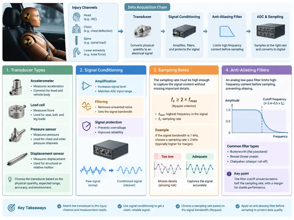
Every injury criterion computed after a crash test — HIC15, 3 ms chest clip, Nij, tibia index, BrIC — is only as trustworthy as the analog signal that entered the data acquisition system. A crash test is a one-shot, destructive event: there is no opportunity to re-measure. This makes the acquisition chain the single most consequential engineering decision in the entire test setup. This chapter establishes the physical and mathematical foundations of that chain: what the transducers actually measure, how their signals are conditioned, how they are sampled, and why the anti-aliasing filter is not an optional accessory but a load-bearing part of the measurement.
Transducer Types and What They Physically Measure
Injury channels fall into a small number of physical families, and each family imposes its own constraints on the acquisition chain.
- Piezoresistive accelerometers — the workhorse for head, chest, and pelvis acceleration. A silicon MEMS or strain-gauge bridge changes resistance under inertial loading. Typical full-scale ranges in crash testing are ±500 g to ±2000 g for head CG sensors, ±200 g to ±500 g for chest and pelvis, with sensitivity expressed in mV/g. They are DC-coupled, so they can measure sustained acceleration (important for rollover and low-speed events), but they are sensitive to thermal zero drift and require a stable bridge excitation supply.
- Piezoelectric accelerometers — used where high-frequency content matters (e.g., component-level impact, some femur/tibia mounts). They are AC-coupled by nature, cannot measure static or very low-frequency acceleration, and require charge amplifiers. Their wide dynamic range and low noise floor make them attractive, but the low-frequency roll-off must be documented because it affects integration to velocity and displacement.
- Load cells and force transducers — strain-gauge bridges measuring belt force, seat force, steering column force, and pedal force. Ranges are typically 5 kN to 20 kN with sensitivities around 1–3 mV/V at full scale.
- Potentiometers and string pots — displacement of the steering column, pedal travel, and belt payout. These are inherently low-bandwidth devices (typically < 50 Hz usable) and must not be sampled as if they were acceleration channels.
- Angular rate sensors and tilt sensors — used for head rotation (BrIC), occupant kinematics, and vehicle body motion. MEMS gyros typically cover ±2000 °/s to ±8000 °/s.
The critical engineering point is that each transducer has a usable bandwidth and a dynamic range, and the conditioning and sampling must be matched to both. A ±2000 g accelerometer with a 10 kHz resonant frequency and a 3 kHz usable band cannot be sampled at 10 kHz "because that's what we always do" without first verifying the anti-aliasing filter corner.
Signal Conditioning: Bridge Excitation, Amplification, and Filtering
Raw transducer outputs are small — a 1 mV/g accelerometer at 100 g produces 100 mV, and a strain-gauge bridge produces a few millivolts at full scale. Signal conditioning performs four jobs: excitation, amplification, filtering, and (for some channels) isolation.
For bridge-type sensors, a regulated DC excitation (typically 5 V or 10 V) is applied, and the differential bridge output is amplified by an instrumentation amplifier with high common-mode rejection. The gain is chosen so that the full-scale transducer output maps to roughly 80–90% of the ADC input range — this preserves resolution without risking clipping on transients. For example, a ±500 g accelerometer with 2 mV/g sensitivity produces ±1.0 V at full scale; with a ±5 V ADC input, a gain of 4 places full scale at ±4.0 V, leaving 20% headroom for overshoot.
Filtering at the conditioning stage is the first line of defense against aliasing. A low-pass filter with a corner frequency below the Nyquist frequency must be placed before the ADC. In practice, most crash DAQ systems use a dedicated anti-aliasing filter module (often a Butterworth or Bessel topology) with a corner at 1/2.5 to 1/3 of the sampling rate, and a steep roll-off (typically 4th to 8th order) so that content above Nyquist is attenuated by at least 60–80 dB before sampling.
Sampling Rate and the Nyquist Criterion in Practice
The Nyquist–Shannon theorem states that a signal must be sampled at more than twice its highest frequency component to be reconstructed without aliasing. For injury channels, the practical rule is stricter: sample at 5–10 times the highest frequency of interest, and ensure the anti-aliasing filter corner is at or below the Nyquist frequency.
SAE J211/1 and ISO 6487 define the channel filter classes (CFC 60, CFC 180, CFC 600, CFC 1000) that govern injury channel bandwidth. A CFC 1000 channel has a −3 dB corner at 1650 Hz, so the sampling rate must be at least 10 kHz to satisfy Nyquist with margin; most labs use 20 kHz for CFC 1000 channels. A CFC 180 channel (corner ≈ 300 Hz) is typically sampled at 2–5 kHz. The table below summarizes the practical mapping.
| Channel class | −3 dB corner (Hz) | Minimum sampling (Hz) | Typical lab sampling (Hz) | Typical use |
|---|---|---|---|---|
| CFC 60 | ≈ 100 | 500 | 1 000 | Displacement, belt payout, low-bandwidth kinematics |
| CFC 180 | ≈ 300 | 1 500 | 2 000–5 000 | Chest acceleration, pelvis acceleration, belt force |
| CFC 600 | ≈ 1 000 | 5 000 | 10 000 | Head acceleration (many OEM specs) |
| CFC 1000 | ≈ 1 650 | 10 000 | 20 000 | Head CG acceleration, high-rate force channels |
Note that the sampling rate is not the same as the filter corner. Sampling at 20 kHz does not mean the channel is valid to 10 kHz; the CFC 1000 filter limits the usable content to roughly 1.65 kHz. The sampling rate exists to capture the filtered signal faithfully, not to extend bandwidth.
Anti-Aliasing: Why It Cannot Be Fixed in Post-Processing
Aliasing is the folding of high-frequency content onto lower frequencies during sampling. Once folded, it is mathematically indistinguishable from genuine low-frequency signal — no digital filter applied after the ADC can remove it. This is why the anti-aliasing filter must be analog and must sit before the sampler.
Consider a head accelerometer channel with a 3 kHz resonance. If the channel is sampled at 10 kHz with no anti-aliasing filter, a 6 kHz component (above Nyquist at 5 kHz) folds to 4 kHz, and a 7 kHz component folds to 3 kHz — directly into the band where HIC is computed. The resulting HIC value can be inflated or deflated by tens of percent, and the error is invisible in the time-domain plot. The figure below shows the acquisition chain and where each defense sits.
Putting It Together: A Practical Channel Setup
Consider a head CG accelerometer channel for a frontal sled test. The transducer is a ±2000 g piezoresistive accelerometer with 0.5 mV/g sensitivity and a 4 kHz mounted resonance. The injury criterion is HIC15, which is governed by CFC 1000 (corner 1650 Hz). The setup proceeds as follows:
- Verify the mounted resonance. A 4 kHz resonance is only 2.4× the filter corner; if the filter roll-off is insufficient, resonance energy can leak into the passband. A 4th-order Bessel at 1650 Hz gives roughly −24 dB at 4 kHz, which is marginal; an 8th-order Butterworth gives −48 dB and is preferred here.
- Set the anti-aliasing corner. Place the analog filter corner at 1650 Hz (CFC 1000) and confirm the stopband attenuation at the Nyquist frequency (10 kHz for a 20 kHz sample rate) exceeds 60 dB.
- Choose the sampling rate. 20 kHz gives 12× oversampling relative to the 1650 Hz corner, which is comfortable and standard for CFC 1000.
- Set the gain. Full scale is ±2000 g × 0.5 mV/g = ±1.0 V. With a ±5 V ADC input, a gain of 4 maps full scale to ±4.0 V, leaving 20% headroom.
- Document the chain. Record transducer serial number, sensitivity, filter type and corner, sample rate, and gain in the channel metadata. This metadata is what allows the post-test analyst to defend the HIC value.
Verification Before the Test
Every channel should be verified with a known input before the test fires. For accelerometers, a shunt calibration or a back-to-back comparison against a reference accelerometer on a shaker provides a gain check. For load cells, a dead-weight or proving-ring calibration confirms the bridge output. The verification should confirm three things: the sensitivity matches the metadata, the channel is not clipping at expected full scale, and the noise floor is below the resolution needed for the injury criterion. A channel that passes all three is ready; a channel that fails any one should be re-conditioned or replaced before the test, because there is no second attempt.
The acquisition chain is the foundation on which every downstream injury interpretation rests. Getting the transducer, conditioning, sampling rate, and anti-aliasing filter right is not paperwork — it is the difference between a defensible injury metric and a number that cannot be trusted.