1. Framing model comparison as an engineeri
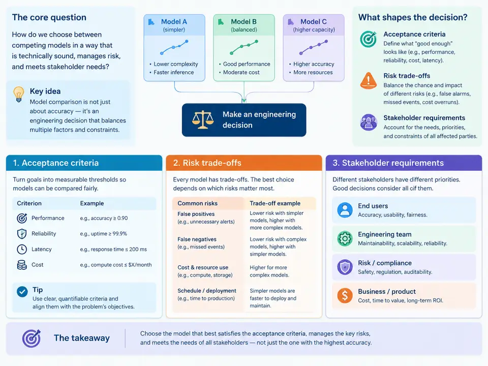
Model comparison is often taught as a statistical ritual: fit several candidates, compute a metric such as RMSE, AIC, or AUC, and declare the winner. In engineering practice this framing is incomplete and frequently misleading. A model is not selected because it scores best in isolation; it is selected because a specific team, under specific constraints, is willing to accept the residual risk of deploying it. The moment you treat model comparison as a decision problem rather than a ranking exercise, three questions become unavoidable: What must the model achieve to be acceptable? What does it cost us when it fails? And who bears that cost?
This chapter establishes the decision-theoretic frame that the rest of the course builds on. We define acceptance criteria as explicit, testable thresholds; we formalize risk trade-offs between error types; and we show how stakeholder requirements translate into constraints on the comparison itself — including which metrics are legitimate, which data splits are admissible, and what evidence must accompany a recommendation.
From "Best Model" to "Acceptable Model"
A ranking answers "which candidate has the lowest expected loss on this sample?" An acceptance decision answers "is any candidate good enough, and which one should we ship given everything we know?" These differ in three structural ways. First, ranking is relative — the best of five poor models is still poor. Second, ranking ignores the cost asymmetry between error types. Third, ranking is silent on uncertainty: a 0.004 AUC advantage computed on 900 validation rows is not evidence of superiority.
The engineering frame replaces a single leaderboard with a decision rule. Formally, let candidate models be \(m_1,\dots,m_k\), let \(\theta\) denote the deployment context (traffic mix, input drift, latency budget), and let \(L(m,\theta)\) be the operational loss. Acceptance requires two conditions:
- Feasibility: \(L(m,\theta) \le L_{\max}\) for the agreed loss definition and confidence level — the model clears the bar at all.
- Selection: among feasible candidates, choose the one minimizing expected loss subject to hard constraints (latency, memory, interpretability, regulatory limits).
Note that feasibility is checked before selection. A model that wins on accuracy but violates a 50 ms p99 latency budget is not a candidate at all; it is a constraint violation. Making this ordering explicit prevents the common failure mode in which a team spends weeks tuning a model that could never have been deployed.
Acceptance Criteria Must Be Operational
An acceptance criterion is only useful if a third party can evaluate it without asking the author what it meant. "The model should be accurate enough" is not a criterion. A workable criterion specifies the metric, the population, the threshold, the uncertainty treatment, and the decision rule when the threshold is narrowly missed. Consider a demand-forecasting service for a parts warehouse:
| Element | Weak phrasing | Operational phrasing |
|---|---|---|
| Metric | "good forecast accuracy" | WMAPE on weekly SKU-level demand |
| Population | "on real data" | rolling-origin backtest, last 26 weeks, SKUs with ≥ 12 nonzero weeks |
| Threshold | "below 20%" | WMAPE ≤ 18% overall and ≤ 30% for the top-50 revenue SKUs |
| Uncertainty | — | upper bound of 90% bootstrap CI on WMAPE ≤ 20% |
| Fallback | — | if overall passes but top-50 fails, escalate to review; do not auto-accept |
The threshold itself should be derived, not invented. Two defensible derivations dominate. The cost-based derivation sets \(L_{\max}\) at the loss of the incumbent process (the current manual forecast, the previous model, or a naive baseline). If the new model cannot beat the status quo's expected cost, it has no business replacing it. The requirement-based derivation starts from a downstream service-level target — for example, "stockout rate ≤ 3%" — and back-solves the forecast error that target tolerates. Both derivations produce a number with a reason attached, which is what makes the criterion negotiable with stakeholders rather than arbitrary.
Risk Trade-offs: The Confusion Matrix as a Cost Table
Every classifier comparison embeds an implicit cost matrix, whether or not anyone wrote it down. Making it explicit is the single highest-leverage step in the entire comparison process. For a fraud-screening model, the two error types are not symmetric:
- False negative (fraud approved): direct loss equal to the transaction amount, plus chargeback fees and reputational damage. In our running example, assume an average realized loss of $340 per missed case.
- False positive (legitimate transaction blocked): customer friction, manual review cost of roughly $12, and a small churn hazard. Assume $18 fully loaded.
The ratio is nearly 19:1. A model with higher accuracy but a worse false-negative rate is worse under this cost structure, even though it wins the leaderboard. This is why threshold selection and model selection cannot be separated: the operating point is part of the model's identity. When comparing candidates, compare them at their cost-optimal thresholds, not at the default 0.5.
Stakeholder Requirements Shape the Comparison Itself
Different stakeholders constrain different parts of the analysis, and ignoring this produces comparisons that are statistically sound and organizationally useless.
- Operations cares about the review queue: a false-positive rate above 4% overwhelms the manual team. This becomes a hard constraint on the operating point, which in turn restricts which models are feasible.
- Compliance and audit may require that the model's decisions be explainable per case. This can eliminate gradient-boosted candidates outright, or require a surrogate explanation layer whose fidelity is itself an acceptance criterion.
- Finance cares about expected loss and variance, not accuracy. A model with slightly higher mean cost but much lower variance may be preferred under a risk-averse mandate.
- Engineering imposes latency, memory, and retraining-cadence constraints that bound the hypothesis class before any data is touched.
The practical consequence is that the comparison protocol — metrics, splits, thresholds, and the evidence package — should be agreed before results are seen. This pre-registration is not bureaucracy; it prevents the well-documented pattern in which the metric is chosen after the fact to favor the model the team already prefers.
Worked Example: Comparing Two Fraud Models Under Asymmetric Cost
Suppose two candidates are evaluated on a held-out validation set of 20,000 transactions containing 400 confirmed frauds. Model A achieves 0.91 AUC; Model B achieves 0.89 AUC. A naive leaderboard picks A. Now apply the cost frame.
At each model's cost-optimal threshold, the confusion matrices (illustrative values for this worked example) are:
| Model | TP | FN | FP | TN | E[C] = 340·FN + 18·FP |
|---|---|---|---|---|---|
| A | 312 | 88 | 640 | 18,960 | 340·88 + 18·640 = $41,440 |
| B | 336 | 64 | 1,180 | 18,420 | 340·64 + 18·1,180 = $43,000 |
Model A wins on expected cost by $1,560, despite the lower AUC — because B's aggressive threshold buys 24 fewer misses at the price of 540 extra false positives, and the arithmetic favors A. But the margin is small relative to sampling noise. A bootstrap over validation rows (1,000 resamples) might yield a 90% interval for the difference of, say, [−$4,900, +$1,800] — straddling zero. The honest conclusion is not "A is better" but "A and B are statistically indistinguishable on cost; select on secondary criteria." Here the operations constraint decides: B's 5.9% false-positive rate exceeds the 4% review-queue limit, so B is infeasible regardless. A ships, and the evidence package records both the cost comparison and the constraint that resolved it.
What the Comparison Must Deliver
Framed as a decision problem, the output of model comparison is not a score but a defensible recommendation with an evidence trail. At minimum it should state: the acceptance criteria and their derivation; the cost matrix and its source; the validation protocol including splits and resampling; each candidate's performance at its cost-optimal operating point with intervals; which constraints eliminated which candidates; and the residual risks the accepting stakeholder is implicitly signing up for. When a comparison cannot clear the bar, a documented no-go with the binding constraint named is a successful outcome — it redirects effort instead of shipping a model that will fail in production. The remaining chapters supply the statistical machinery — proper scoring rules, resampling schemes, significance tests, and calibration checks — that makes each element of this evidence trail rigorous.