1. Quantile Regression for Prediction Inter
Why quantile regression for intervals
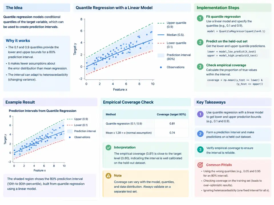
Ordinary least squares estimates the conditional mean, so a single fitted line tells you nothing about the spread of the target around that mean. Quantile regression instead estimates a conditional quantile: fitting the model at the 0.05 and 0.95 quantiles yields a lower and an upper bound that, by construction, should bracket roughly 90% of future observations. This is the appeal for prediction intervals — the bounds are produced directly by the model, they can widen or narrow as a function of the features (heteroscedasticity), and they do not assume Gaussian residuals.
The estimator minimizes the pinball loss (also called the check loss) for a target quantile level τ:
ρ_τ(r) = r · τ        if r ≥ 0
ρ_τ(r) = r · (τ − 1)   if r < 0

minimize  Σ_i ρ_τ( y_i − x_iᵀ β )  +  λ ‖β‖₂
For a symmetric interval at coverage level 1 − α, fit two models: τ_lo = α/2 and τ_hi = 1 − α/2. With α = 0.10 that is τ_lo = 0.05 and τ_hi = 0.95. The interval for a new point x is [xᵀβ_lo, xᵀβ_hi]. Note the two fits are independent — nothing forces the lower bound below the upper bound, so a sanity check on ordering is part of the workflow.
Worked implementation
The example below uses a synthetic dataset with deliberately heteroscedastic noise so that a constant-width interval would be visibly wrong. All numbers are reproducible from the seed; they are illustrative, not measured results.
import numpy as np
from sklearn.linear_model import QuantileRegressor
from sklearn.model_selection import train_test_split

rng = np.random.default_rng(42)
n = 2000
X = rng.uniform(-3, 3, size=(n, 2))
# true conditional mean and a noise scale that grows with |x0|
mu = 1.5 * X[:, 0] - 0.8 * X[:, 1] + 2.0
sigma = 0.4 + 0.6 * np.abs(X[:, 0])
y = mu + rng.normal(0, sigma)

X_tr, X_te, y_tr, y_te = train_test_split(X, y, test_size=0.3, random_state=0)

alpha = 0.10
lo = QuantileRegressor(quantile=alpha / 2, alpha=0.0, solver="highs").fit(X_tr, y_tr)
hi = QuantileRegressor(quantile=1 - alpha / 2, alpha=0.0, solver="highs").fit(X_tr, y_tr)

lower = lo.predict(X_te)
upper = hi.predict(X_te)
covered = (y_te >= lower) & (y_te <= upper)
print("empirical coverage:", covered.mean())
print("mean width:", (upper - lower).mean())
print("ordering violations:", (upper < lower).sum())
Two details matter for reproducibility. First, solver="highs" is required by recent scikit-learn versions for the linear-programming formulation; the default may raise or fall back depending on version. Second, alpha=0.0 disables the L2 penalty so the fit matches the plain pinball-loss objective above — set a small positive value only if you actually want regularization.
Reading the coverage result
Empirical coverage is the fraction of held-out points whose true y falls inside [lower, upper]. For a nominal 90% interval on a few hundred test points, sampling noise alone moves the estimate by roughly ±2–3 percentage points, so treat a result in the 0.87–0.93 band as consistent with the target. A value far below 0.90 signals under-coverage: the quantile fits are too tight, often because the model is misspecified (missing interaction or nonlinear term) or because the training and test distributions differ. A value far above 0.90 with very wide intervals signals over-coverage and poor efficiency — the bounds are valid but uninformative.
Mean width is the efficiency counterpart: two models can both hit 90% coverage while one produces intervals twice as wide. Always report coverage and width together, and inspect width as a function of the features to confirm the model is capturing heteroscedasticity rather than emitting a near-constant band.
lower = min(lower, upper) is acceptable for reporting, but investigate first — persistent violations suggest the two quantile levels are too close or the sample is too small for stable tail fits.Interval structure across the feature space
The diagram below shows how the two fitted quantile surfaces combine into a prediction band whose width changes with the input, which is the property that motivates quantile regression over a constant-width residual interval.
Verification checklist
- Coverage on held-out data — compute
((y_te >= lower) & (y_te <= upper)).mean(); expect ≈ 0.90 for α = 0.10, allowing for test-set sampling noise. - Width distribution — report mean and interquartile range of
upper − lower; a near-zero spread means the model is not adapting to the features. - Ordering — count
(upper < lower).sum(); should be zero or negligible. - Calibration across subgroups — split the test set by a feature (e.g.
x₀ < 0vsx₀ ≥ 0) and check coverage in each; systematic gaps reveal misspecification. - Baseline comparison — compare against a constant-width interval from residual quantiles of an OLS fit; quantile regression should match coverage while reducing width where the conditional spread is smaller.
Common failure symptoms
| Symptom | Likely cause | Action |
|---|---|---|
| Coverage ≈ 0.75 at nominal 0.90 | Model misspecified; missing nonlinear term or interaction | Add features or use a nonlinear quantile model; re-check residual patterns |
| Coverage ≈ 0.98 with very wide band | Over-conservative tail fits; small sample or heavy regularization | Increase sample size, reduce alpha, inspect tail quantile stability |
| Frequent ordering violations | Quantile levels too close or too few observations in the tails | Widen α, pool data, or fit a single model with monotonic constraints |
| Constant band width | Features carry no information about spread | Expected if homoscedastic; otherwise add spread-relevant features |
The core deliverable of this case is a fitted pair of quantile models plus a coverage-and-width report on held-out data. Once that report is stable, the interval is ready to be compared against resampling or conformal alternatives on the same split.