1. Course overview

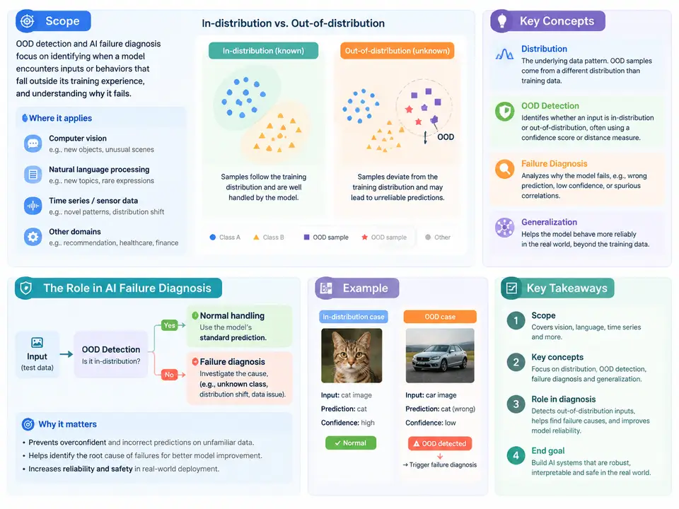
Machine learning systems deployed in the real world rarely encounter only the data distribution they were trained on. A road-scene classifier trained on daytime urban footage will eventually meet fog, snow, or a construction detour; a medical imaging model trained on one scanner vendor will encounter images from another; a fraud detector trained on last year's transaction patterns will face new attack strategies. When inputs drift away from the training distribution, model confidence often stays high while accuracy collapses — a failure mode that is silent, systematic, and expensive. Out-of-distribution (OOD) detection is the discipline of identifying inputs that do not belong to the distribution a model was trained to handle, and it is the first line of defense in AI failure diagnosis: the practice of detecting, localizing, explaining, and remediating the ways a deployed model fails.

This course treats OOD detection not as an isolated benchmark task but as an operational capability embedded in a larger diagnostic loop. Across 30 chapters, you will move from the conceptual foundations (what "distribution" means operationally, how OOD differs from anomaly, novelty, and adversarial input) through concrete detection methods (softmax-based scores, energy and logit-based scores, distance-based and density-based approaches, Bayesian and ensemble uncertainty, reconstruction-based detectors), and then into the diagnostic layer: root-cause analysis, data slicing, drift attribution, calibration, monitoring, and incident response. The goal is practical fluency — the ability to look at a failing model in production, decide whether the failure is distributional, label-related, or architectural, and choose a detection and mitigation strategy that fits the cost structure of the application.

Core concepts and how they relate

Precision matters here, because these terms are frequently conflated in practice. The in-distribution (ID) set is the data a model was trained and validated on, characterized by a joint distribution P(x, y) over inputs and labels. Out-of-distribution inputs are drawn from a different distribution Q(x) — either a covariate shift (same label semantics, different input statistics, e.g., a new camera sensor) or a semantic shift (inputs from classes the model was never trained to recognize, e.g., a pedestrian detector encountering a horse). Anomalies are rare events within the operational data stream; they may be ID or OOD. Novelty detection is typically a one-class problem: learn the boundary of normal data and flag anything outside it. Open-set recognition extends classification to reject unknown classes at inference time. Adversarial examples are deliberately perturbed inputs that are technically near the ID distribution but cause misclassification — a distinct threat model that OOD detectors are not designed to catch.

The practical distinction that matters most for diagnosis is what signal you have available. If you have labels for the new data (even delayed), you can measure accuracy directly and attribute failures to specific classes. If you have only unlabeled inputs, you must rely on distributional scores. If you have neither — the common production case — you need a monitoring pipeline that computes OOD scores continuously and escalates when they cross thresholds calibrated on held-out ID data.

Where OOD detection sits in the failure-diagnosis workflow

A useful mental model is a four-stage diagnostic loop: detect (is something wrong?), localize (which inputs, classes, or slices are affected?), explain (what kind of distributional change is it — covariate, semantic, label noise, or adversarial?), and remediate (retrain, recalibrate, add a rejection class, or route to human review). OOD detection primarily serves the first two stages, but its outputs — score distributions, threshold crossings, per-slice OOD rates — are the raw material for the explanatory stage. A spike in energy scores concentrated on night-time images points to covariate shift; a spike spread uniformly across classes with high semantic-shift scores points to novel object categories entering the scene.

The diagram below shows this diagnostic loop and the signal paths that connect a deployed model's outputs to each stage. Note that the OOD score is computed from the model's own logits or features — no external labels are required — which is what makes continuous monitoring feasible.

A worked example: catching a silent failure

Consider a concrete scenario that will recur throughout the course. A binary image classifier for product-defect inspection is trained on 50,000 images from a single production line, achieving 98.2% validation accuracy. Three months after deployment, the line adds a second camera with a different color profile. The model still outputs confident predictions — mean max-softmax probability stays around 0.94 — but the true defect-detection rate on the new camera's images drops to 71%. No alert fires, because the model has no mechanism to know it is wrong.

Now add an OOD score. Using the energy score E(x) = -T · logsumexp(z / T) with temperature T = 1, computed from the model's logits, we calibrate a threshold on a held-out ID set such that 95% of ID inputs fall below it. On the new camera's images, the OOD rate jumps from 4.8% (ID baseline) to 38%. That jump is the diagnostic signal: it tells us the new inputs are distributionally different before we have any labels. Slicing by camera reveals the effect is concentrated entirely on the new device, ruling out a global model regression. The remediation is then targeted — either recalibrate the color profile, fine-tune on a small labeled sample from the new camera, or route high-OOD-score images to human review until retraining completes.

This example illustrates the central claim of the course: OOD detection converts a silent accuracy failure into an observable, localizable signal. It does not tell you why the distribution shifted or what to do about it — that is the job of the diagnostic stages that follow — but without it, the failure remains invisible until it surfaces as a business incident.

What you will be able to do

By the end of the course, you should be able to: select an OOD scoring method appropriate to your model architecture and latency budget; calibrate thresholds with explicit false-positive/false-negative trade-offs; build a monitoring pipeline that computes scores on unlabeled production data; distinguish covariate from semantic shift using score distributions and feature-space analysis; and integrate OOD signals into an incident-response workflow with clear escalation criteria. The chapters are sequenced so that each builds on the previous one's operational vocabulary, and every method is presented with the inputs it requires, the computation it performs, and the failure symptoms it is and is not suited to detect.