1. Course overview
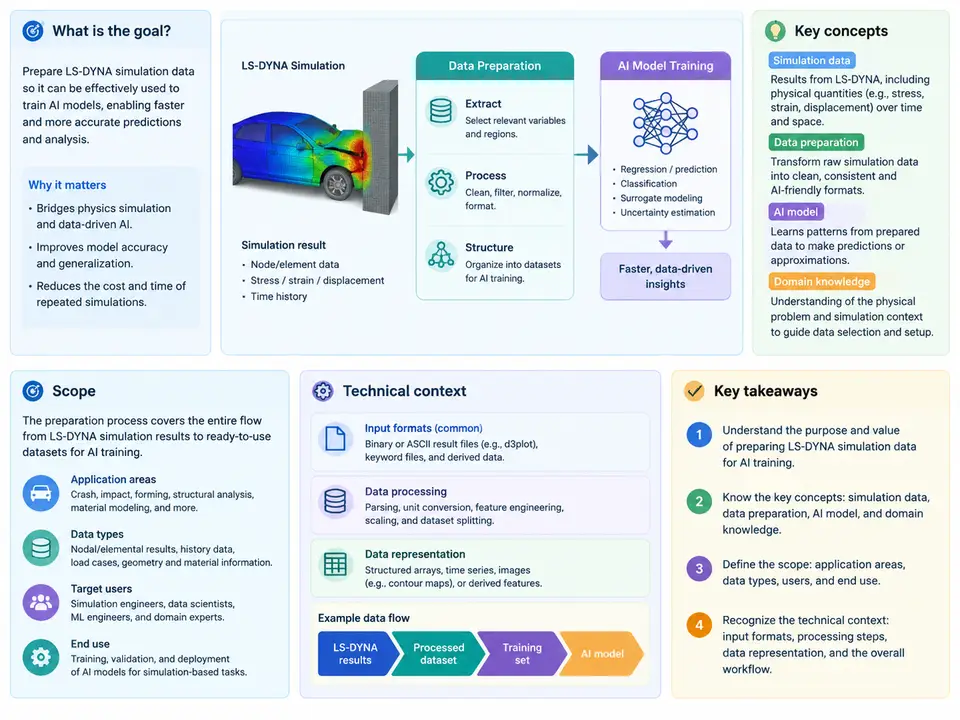
Crash simulation has always produced large volumes of numerical output, but the rise of data-driven engineering has changed what that output is for. Instead of serving only a single design decision, LS-DYNA results are now increasingly treated as training material: curated, labeled, and structured so that surrogate models, anomaly detectors, and reduced-order models can learn from them. This course is about that transformation — the engineering discipline of turning raw LS-DYNA simulation artifacts into datasets that are trustworthy enough to train AI models on.
The scope is deliberately narrower than "machine learning for CAE" and broader than "exporting d3plot files." It covers the full preparation pipeline: defining what the model must learn, designing simulation campaigns that produce informative samples, extracting and normalizing field and scalar data, attaching physically meaningful labels, splitting and versioning datasets, and validating that the resulting data is fit for training. LS-DYNA is the source system throughout, but the concepts transfer to other explicit solvers.
Why LS-DYNA data needs dedicated preparation
LS-DYNA output is engineered for post-processing by humans and by visualization tools, not for consumption by learning algorithms. Several properties make naive reuse problematic:
- Heterogeneous formats. A single run may produce
d3plot(binary state database),binout(time-history channels),nodout/elout(ASCII nodal and element output),glstat/matsum(global and material energy summaries), andrcforc(contact forces). Each has its own reader, sampling behavior, and precision. - Mesh-dependent dimensionality. Nodal and element fields live on a mesh whose node and element counts differ between models. A neural network cannot consume variable-length vertex lists without a canonicalization step — remeshing, resampling onto a reference grid, or graph construction.
- Units and coordinate conventions. LS-DYNA is unit-agnostic; the analyst chooses a consistent system (commonly mm–ms–kg–kN or m–s–kg–N). Mixing runs from different unit systems without conversion silently corrupts every learned relationship.
- Time discretization. Explicit runs use variable critical time steps. Output intervals are controlled by
*DATABASE_BINARY_D3PLOT(DT) and ASCII output intervals by*DATABASE_ASCII_*. Two runs of the same model can yield different state counts. - Class imbalance and redundancy. Most timesteps of a crash event are uneventful; the informative physics is concentrated around impact, buckling onset, and failure. Uniform sampling wastes capacity on near-duplicate frames.
The preparation pipeline at a glance
The diagram below shows the end-to-end data flow and, importantly, the feedback loops that distinguish a serious dataset effort from a one-off export script. Requirements flow forward; quality findings flow backward and force campaign redesign.
Core concepts and vocabulary
Four terms recur throughout the course and are worth fixing now.
Sample. One training example. In crash learning this is rarely a whole simulation; it is usually a (geometry, material, load-case) parameter vector paired with a response — a scalar such as peak intrusion or maximum acceleration, a time series at a sensor location, or a field on a canonical mesh. Deciding the sample granularity is the first design decision, because it determines how many independent runs you need.
Design of experiments (DOE). The parameter space sampling plan. A Latin hypercube over five thickness and material parameters with 120 runs gives better coverage than 120 hand-picked variants. LS-DYNA's *PARAMETER and *INCLUDE structure makes parametric runs straightforward: a template keyword deck plus a parameter file per run.
Canonical representation. The fixed-shape tensor or graph that the model consumes. For scalar surrogates this is trivial; for field prediction it requires a reference mesh, a resampling operator, and a documented node ordering. Canonicalization must be deterministic and versioned, because a silent change in node ordering invalidates every previously trained model.
Leakage. The failure mode where information from validation or test runs influences training. In simulation data the usual culprits are near-duplicate runs (same geometry, slightly different timestep) landing in different splits, and normalization statistics computed over the full dataset before splitting.
A concrete example: intrusion surrogate for a front rail
Consider a simplified but realistic task: predict peak longitudinal intrusion of a front crash rail as a function of three design variables — rail gauge t (1.4–2.4 mm), yield stress σy (280–420 MPa), and impact velocity v (40–64 km/h). The unit system is mm–ms–kg–kN, so stress is in GPa·10³ and velocity in mm/ms.
A workable campaign uses a 60-point Latin hypercube. Each run is generated from a template deck by substituting parameters:
*PARAMETER
t_gauge     , 1.80
sig_yield   , 350.0
v_impact    , 15.0
*INCLUDE
rail_mesh.k
rail_material.k
*DATABASE_BINARY_D3PLOT
$#   dt    lcdt    beam    nplt
   0.50       0       0      50
*DATABASE_ASCII_NODOUT
$#   dt
   0.10
*DATABASE_GLSTAT
$#   dt
   0.10
*END
After solving, extraction reads binout for the rail tip node's displacement history and glstat for the hourglass and total energy ratio. The label is the maximum of the axial displacement component over the event window. A run is rejected if the hourglass-to-total-energy ratio exceeds 5% or if the model shows negative volume errors — both are symptoms that the numerical result is not physically meaningful and should not become a training label.
With 60 runs, a gradient-boosted regressor or a small MLP typically reaches R² around 0.9 on held-out runs if the split is by run and normalization is fit on the training fold only. This is an illustrative expectation for a well-conditioned problem, not a guaranteed result; the actual figure depends on how nonlinear the intrusion response is over the sampled range.
What "good" data preparation looks like
Three properties separate a dataset that supports credible models from one that produces impressive-looking but fragile results. Traceability: every sample can be traced to a specific keyword deck, solver version, and extraction script revision. Physical validity: energy balance, hourglass control, and termination status are checked before a run enters the dataset. Documented coverage: the parameter ranges and the sampling density are recorded, so that model predictions outside the training envelope are flagged rather than trusted.
The remaining chapters build each stage of the pipeline in detail: keyword-level control of output, binary and ASCII extraction with LS-PrePost and Python tooling, mesh canonicalization, labeling strategies for scalar and field targets, dataset splitting and versioning, and validation protocols that catch leakage and coverage gaps before they reach a trained model.