1. Role of LS-DYNA in AI training data gene
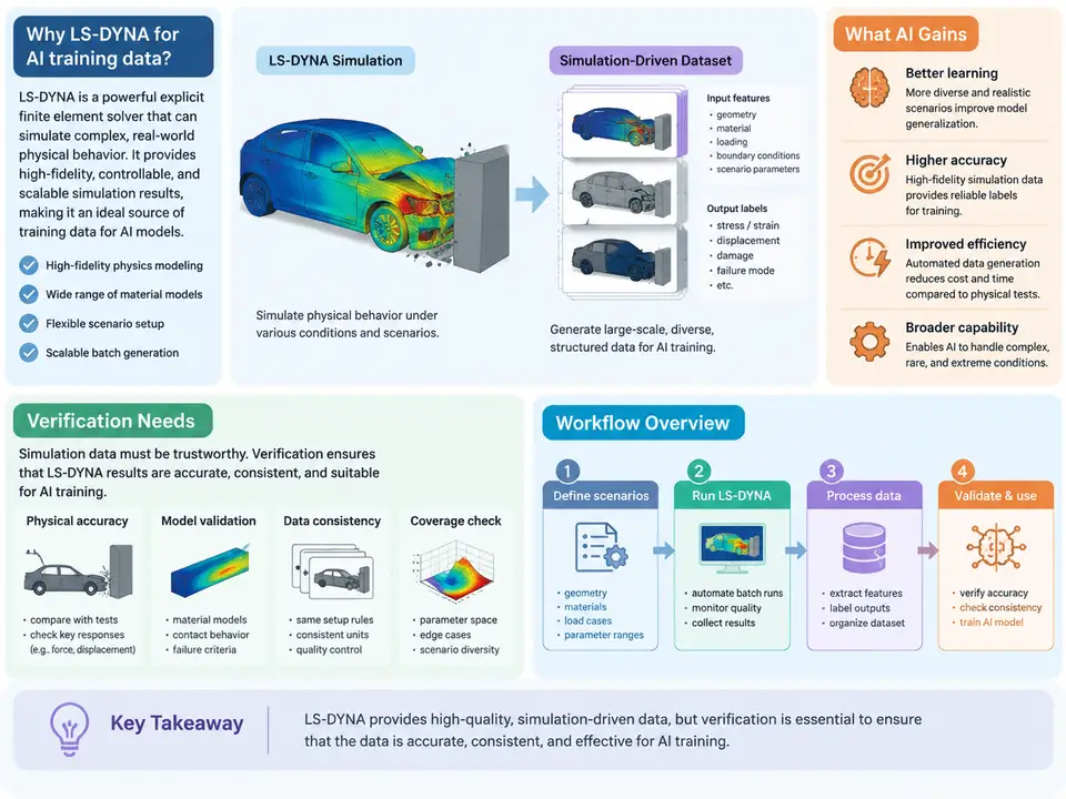
Machine-learning models that reason about crashworthiness, impact, and structural failure need training data that reflects the physics of high-rate, large-deformation events. Physical crash tests are expensive, sparse, and difficult to instrument densely; real-world accident data is noisy and biased toward specific configurations. LS-DYNA fills this gap by acting as a high-fidelity physics oracle: an explicit finite-element solver whose outputs can be sampled at scale to produce labeled datasets for surrogate models, perception pipelines, and anomaly detectors. This chapter establishes why LS-DYNA is used for dataset generation, what verification the resulting data requires, and how the end-to-end workflow is structured.
Why Simulation-Driven Datasets
An AI model trained on LS-DYNA output learns the mapping between a design or loading configuration and a response field — for example, predicting occupant compartment intrusion from a set of barrier-impact parameters, or estimating peak acceleration at a sensor location from vehicle topology. The solver provides three properties that raw test data cannot match at scale: dense spatial and temporal sampling (every element, every timestep), controlled parameter sweeps (vary one input while holding others fixed), and ground-truth access (internal energies, contact forces, and material state are directly available rather than inferred).
The trade-off is that simulation output is only as trustworthy as the model behind it. A dataset generated from an unvalidated deck teaches the AI the solver's artifacts as if they were physics. This is why verification is not an afterthought but a first-class stage of the data-generation pipeline.
What Verification Must Cover
Verification for AI training data operates at three levels, and each produces a different kind of evidence:
- Numerical verification — is the simulation converged and stable? Check energy balance (hourglass and internal energy ratios), timestep stability, and mesh convergence. A run whose hourglass energy exceeds roughly 5–10% of internal energy is a candidate for exclusion or re-meshing.
- Physical validation — does the model reproduce known reference behavior? Compare against physical test data (accelerometer traces, intrusion measurements) or analytical benchmarks. Validation establishes that the deck's constitutive models and contacts are credible.
- Data-quality verification — are the extracted labels consistent, complete, and free of solver artifacts? This includes checking for unphysical spikes, negative volumes, and inconsistent units across the dataset.
Workflow Overview
The pipeline from a parametric model to a verified dataset has five connected stages. The diagram below shows the data and control flow, including the feedback loop where failed verification returns runs to the parameter-sweep stage rather than discarding the whole batch.
Each stage has a concrete artifact. The parametric model is a keyword deck with parameterized dimensions and material properties. The sweep stage produces a design-of-experiments matrix — for a frontal-impact study, this might vary bumper thickness (1.8–3.2 mm), rail gauge (1.2–2.0 mm), and impact velocity (40–64 km/h) across 200 runs using a Latin hypercube. The solve stage executes each run, typically in MPP mode across a compute cluster, writing d3plot and binout files. The extraction stage converts those binary outputs into tabular or tensor labels: peak intrusion per node, acceleration time histories resampled to a fixed rate, and scalar energy metrics. The verification stage filters runs before they enter the dataset.
A Concrete Extraction Example
Consider extracting a single label — peak longitudinal acceleration at a sensor node — from a completed run. The binout file stores nodal acceleration under the nodout channel. A minimal extraction step in Python using lasso-python (LS-DYNA's Python reader) looks like this:
import lasso
d3plot = lasso.dyna.D3plot("run_042/d3plot")
# node 1050 is the B-pillar sensor location
acc = d3plot.get_node_acceleration(node_ids=[1050])
peak_g = acc.max() / 9810.0   # mm/s^2 -> g
print(f"peak acceleration: {peak_g:.2f} g")
The extracted value is only usable if the run passed verification. A peak of 85 g from a run whose hourglass energy reached 14% of internal energy is a solver artifact, not a physical prediction, and must be excluded. This is the essential discipline of simulation-driven dataset generation: every label carries a verification provenance.
Failure Modes and Their Symptoms
Three failure patterns dominate early attempts at LS-DYNA dataset generation, and each has a recognizable symptom:
| Failure mode | Symptom | Typical remedy |
|---|---|---|
| Hourglassing | Hourglass energy > 10% of internal energy; checkerboard deformation in d3plot | Switch to fully integrated elements or add hourglass control (type 4/5) |
| Timestep collapse | Termination before physical end time; smallest element controls dt | Mass scaling with a documented added-mass budget (< 2%) |
| Contact instability | Penetration spikes, negative volumes near interfaces | Adjust penalty stiffness, add segment-based contact |
When a batch shows a cluster of failures in one parameter region — say, all runs with rail gauge below 1.4 mm — the correct response is to inspect that region's decks rather than to discard the runs silently. The failure pattern itself is information about the model's valid envelope.
What the Dataset Must Carry Forward
A verified dataset is more than a table of inputs and outputs. Each record should retain the parameter vector, the extracted labels, the verification metrics (hourglass ratio, energy error, termination status), and a reference to the source run directory. This provenance lets downstream training distinguish in-envelope from extrapolated samples and lets auditors trace any label back to its d3plot. The workflow described here — parametric model, sweep, solve, extract, verify — is the backbone that every later chapter refines: meshing strategy, material calibration, contact tuning, and label schema design all plug into these five stages.