1. Crash deformation prediction landscape
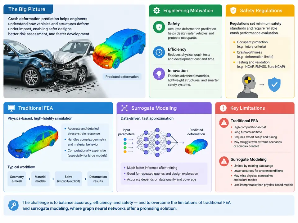
Every vehicle body structure is, at its core, a life-safety device. When a passenger car strikes a rigid barrier at 64 km/h, the front longitudinal rails, crash boxes, and shotgun structures must absorb on the order of 100–200 kJ of kinetic energy within roughly 60–100 ms, while keeping the passenger cell intrusion below thresholds that protect occupants. Predicting exactly how that metal folds, buckles, and tears is one of the most consequential engineering problems in automotive development — and one of the most computationally demanding.
This chapter establishes the landscape: why deformation prediction matters, what regulations constrain it, and where the two dominant traditional approaches — explicit finite element analysis (FEA) and data-driven surrogate modeling — fall short. Understanding these limitations is the motivation for the graph-based methods developed throughout the rest of this course.
Engineering Motivation: Why Deformation Prediction Is Hard
Crashworthiness design is a multi-objective optimization problem played out over a highly nonlinear, rate-dependent, large-deformation regime. The structure must be stiff enough to transmit loads efficiently during normal operation, yet collapse in a controlled, progressive manner during impact. The energy-absorbing members must fold in a stable sequence — crash box first, then longitudinal rail, then firewall — rather than buckling catastrophically or bending globally.
Three engineering realities make this difficult:
- Nonlinearity and path dependence. Sheet metal undergoing plastic folding exhibits strain-rate sensitivity, strain hardening, and failure initiation that depend on the entire loading history. A rail that folds cleanly at 50 km/h may tear at 64 km/h because the fold radius exceeds the material's forming limit.
- Geometric complexity. A modern body-in-white contains thousands of stamped panels, spot welds, adhesive bonds, and extruded sections. The load path through this assembly is not obvious from geometry alone; it emerges from the interaction of connected components.
- Design-space explosion. Gauge thickness, material grade, bead patterns, weld spacing, and section geometry all interact. A typical front-end crashworthiness study may involve 20–50 design variables, and the feasible region is narrow and non-convex.
The practical consequence is that engineers need predictions fast enough to iterate on design, accurate enough to trust for safety-critical decisions, and interpretable enough to explain why a structure behaves as it does.
Safety Regulations: The Constraints That Define the Problem
Deformation prediction is not an academic exercise; it is bounded by regulatory and consumer-test requirements that specify impact conditions, occupant injury criteria, and structural performance thresholds. The table below summarizes the principal load cases that drive body-structure design in most global markets.
| Load case | Typical condition | Primary structural metric | Regulatory / rating context |
|---|---|---|---|
| Full frontal rigid barrier | 56 km/h, 100% overlap | B-pillar / pedal intrusion, occupant deceleration | FMVSS 208, UN R94 |
| Offset deformable barrier (ODB) | 64 km/h, 40% overlap | Toe pan intrusion, A-pillar rotation | Euro NCAP, UN R94 |
| Small overlap frontal | 64 km/h, 25% overlap | Wheelhouse intrusion, hinge-pillar integrity | IIHS |
| Side impact barrier | 50–60 km/h, mobile deformable barrier | B-pillar intrusion velocity, door trim penetration | FMVSS 214, UN R95, Euro NCAP |
| Rear impact | 80 km/h, 70% overlap | Fuel system integrity, seatback strength | FMVSS 301 |
Each load case imposes a different deformation mode. The full frontal case rewards symmetric, progressive folding of both rails; the small overlap case loads the structure outboard of the rails and demands that the wheelhouse and hinge pillar carry load through a path never intended as primary. A prediction method must therefore resolve not just how much deformation occurs but where and in what sequence — the spatial distribution of plastic strain and the timing of fold formation.
Traditional FEA: The Reference Method and Its Costs
Explicit dynamic FEA is the industry reference. A full-vehicle crash model discretizes the body into 5–15 million shell elements, applies contact definitions across hundreds of interacting parts, and integrates the equations of motion with an explicit central-difference scheme at a stable time step governed by the smallest element size (typically 0.5–1.0 μs). A 150 ms simulated event therefore requires 150,000–300,000 time steps.
The workflow is well established: build the mesh, assign material cards (e.g., *MAT_024 for elastoplastic steel with strain-rate curves), define contacts and spot welds, prescribe initial velocity and boundary conditions, and run on a cluster. A single 64 km/h ODB simulation on 64–128 cores takes roughly 8–24 hours wall-clock. That cost is acceptable for verification, but it is prohibitive for design exploration: a 50-variable DOE with 500 runs would consume 5,000–12,000 core-hours per iteration loop.
Beyond cost, FEA has three structural limitations for prediction-centric workflows:
- Mesh dependence and modeling burden. Results shift with element size, hourglass control, and weld representation. Building a trustworthy model is itself a multi-week expert task, and each geometry change requires re-meshing and re-validation.
- Poor suitability for gradient-based optimization. The response is noisy and non-differentiable with respect to design variables; finite-difference gradients require many perturbed runs.
- Limited transferability. A model tuned for one platform does not transfer to a new architecture without re-validation, so knowledge does not accumulate across programs.
Surrogate Modeling: Faster, but Structurally Blind
Surrogate models address the cost problem by fitting a cheap approximation to a set of FEA samples. Common choices include polynomial response surfaces, Kriging/Gaussian processes, radial basis functions, and — more recently — neural networks. Given a design vector x (thicknesses, grades, bead parameters), the surrogate predicts scalar responses such as peak intrusion or energy absorbed.
The limitation is fundamental: conventional surrogates operate on global design descriptors and produce global or low-dimensional outputs. They can tell you that a 0.2 mm gauge increase on the front rail reduces toe-pan intrusion by 8 mm, but they cannot tell you which portion of which panel carries the load, where a fold initiates, or how the deformation pattern changes when a weld fails. The spatial field — the actual deformation — is collapsed into a handful of scalars, discarding exactly the information engineers need to diagnose and redesign.
Attempts to predict full deformation fields with CNNs or voxel networks exist, but they impose a grid structure on irregular geometry, require large labeled datasets, and generalize poorly across topology changes. The core mismatch is representational: crash structures are graphs — nodes are joints, weld points, and element centroids; edges are structural connections and load paths — yet traditional surrogates treat them as vectors or images.
Where Graph Neural Networks Fit
The gap is now precise. Engineers need a predictor that (1) runs in seconds to minutes, (2) outputs spatially resolved deformation rather than scalars, (3) respects the connectivity and load-path structure of the body, and (4) transfers across geometries. Graph neural networks address all four: they operate directly on mesh- or component-level graphs, propagate information along edges (load paths), and produce per-node outputs (nodal displacement, plastic strain) that reconstruct the deformation field.
The figure below maps the landscape: the two traditional pillars, their cost and fidelity trade-offs, and the representational gap that graph-based methods occupy.
What This Course Builds Toward
The remainder of the course develops the graph-learning machinery needed to close this gap. You will learn how to construct structural graphs from crash models (nodes as element clusters or joints, edges as welds, adhesives, and contact pairs), how to encode node and edge features (thickness, material grade, section properties, relative position), and how message-passing networks can be trained on FEA-generated datasets to predict nodal displacement and plastic strain fields. The evaluation standard is deliberately strict: a useful model must reproduce intrusion metrics within engineering tolerance and produce deformation fields whose fold locations and sequence match the reference simulation.
The starting point for any such effort is a clear-eyed view of the baseline. FEA remains the ground truth and will generate the training data; scalar surrogates define the performance bar that graph methods must beat on spatial resolution. With the motivation, regulatory constraints, and baseline limitations established, the next chapter turns to the graph representation itself — how a crash structure becomes a learnable object.