1. Course overview
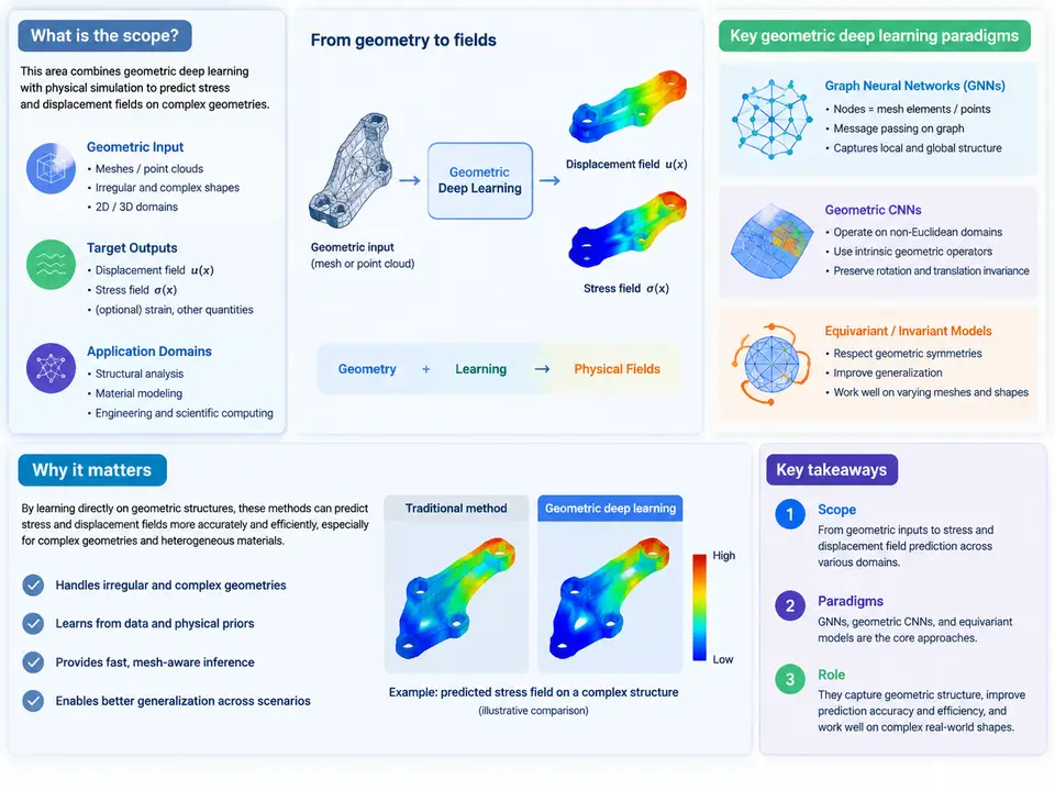
Predicting how a structure deforms and how stress distributes through its material is one of the oldest and most consequential problems in engineering mechanics. Classical approaches — analytical solutions for canonical geometries, and the finite element method (FEM) for everything else — remain the backbone of structural analysis. Yet a growing class of problems exposes their limits: real-time digital twins, inverse identification from sparse sensor data, topology optimization loops that require thousands of field evaluations, and surrogate modeling where a single high-fidelity simulation may cost hours. This course addresses those problems through geometric deep learning (GDL): a family of neural architectures designed to respect the symmetries, invariances, and local connectivity that govern physical fields on geometric domains.
The scope of the course is deliberately narrow in physics and broad in method. On the physics side, we focus on two coupled field quantities — the displacement field u(x) and the stress field σ(x) — over two- and three-dimensional continua, together with the constitutive and equilibrium relations that bind them. On the method side, we cover the principal GDL paradigms: graph neural networks (GNNs) on meshes and point clouds, convolutional and spectral operators on regular grids, neural operators (Fourier neural operators, deep operator networks) that map between function spaces, and physics-informed neural networks (PINNs) that embed governing equations as soft constraints. The unifying thread is that each architecture encodes a prior about geometry and symmetry, and that prior determines what the model can learn from limited data.
Why geometry demands its own learning paradigm
A stress field is not an arbitrary function of coordinates. It obeys balance of momentum, ∇·σ + b = 0 in the static case; it is tied to strain through a constitutive law, σ = C : ε for linear elasticity; and strain derives from displacement via ε = ½(∇u + ∇uT). These relations are equivariant under rigid-body motion: rotate the body and the fields rotate with it; translate it and the fields translate. A model that ignores this symmetry must waste capacity relearning it from data. GDL architectures build the symmetry in by construction — message passing over local neighborhoods, rotation-equivariant features, or operator kernels that commute with translation.
Equally important is discretization independence. A mesh with 4,000 nodes and one with 40,000 nodes describe the same continuum. A useful surrogate should transfer across resolutions, or at least degrade gracefully. Graph-based and operator-based models are designed with this in mind, whereas a plain multilayer perceptron trained on flattened nodal coordinates is not.
The four paradigms at a glance
The diagram below positions the main paradigms along two axes that matter in practice: how the geometry is represented (mesh/graph versus continuous function space) and how physics enters the model (purely data-driven versus equation-constrained).
Reading the map: graph neural networks sit in the discrete, data-driven corner and are the natural choice when you already have an FE mesh and abundant simulation labels. Physics-informed GNNs add equilibrium residuals to the loss, trading training complexity for label efficiency. Neural operators move to the continuous side, learning mappings between function spaces so that a single trained model can be queried at any resolution. Physics-informed operators combine both advantages but are the most demanding to stabilize. PINNs, shown at the center, are pointwise and mesh-free — useful for inverse problems and irregular domains, but expensive to train for large 3D fields.
What the course will actually build
Each paradigm is introduced with a concrete engineering task rather than an abstract benchmark. Early chapters use a cantilever beam and a plate with a hole under plane stress, where analytical or high-fidelity FE reference solutions are available for validation. Later chapters move to 3D solid mechanics, contact, and heterogeneous materials. A representative data pipeline for a GNN surrogate looks like this:
# Example: assembling a mesh-graph dataset from FE runs (illustrative parameters)
# Geometry: 2D plate with circular hole, plane stress, unit thickness
# Material: E = 210 GPa, nu = 0.3, linear elastic
# Load cases: uniaxial tension sigma_x in {50, 100, 150, 200} MPa
# Mesh: ~3,200 triangular elements, ~1,650 nodes per sample

for load in [50, 100, 150, 200]:
    solve_fem(geometry="plate_hole", E=210e3, nu=0.3, sigma_x=load)
    nodes  = extract_nodal_coordinates()      # shape (N, 2)
    edges  = extract_mesh_connectivity()      # shape (2E, 2)
    u_true = extract_nodal_displacement()     # shape (N, 2)
    s_true = extract_element_stress()         # shape (M, 3) in Voigt notation
    save_sample(nodes, edges, load, u_true, s_true)
Two conventions must be fixed before any training begins, and they are stated once here and held for the entire course. First, sign convention: tensile stress is positive, and displacement components are positive along the global x and y axes. Second, normalization: nodal coordinates are scaled to the unit box, displacements are divided by a characteristic length, and stresses by the applied load magnitude, so that loss terms from different field quantities are comparable. Inconsistent conventions are the single most common source of silently wrong surrogates.
How to judge whether a surrogate is any good
Field prediction accuracy cannot be summarized by a single scalar without care. Throughout the course we report, at minimum: relative L2 error on displacement, relative L2 error on the von Mises stress, and the maximum absolute error at the stress concentration (the hole boundary in the plate example), because global metrics hide localized failures precisely where engineers care most. A model that achieves 2% global stress error but 25% error at the notch is not usable for fatigue assessment. We also test extrapolation — training on loads up to 150 MPa and evaluating at 200 MPa — since interpolation-only performance is a weak claim.
Prerequisites and expected outcomes
Readers should be comfortable with linear elasticity, the basics of the finite element method, and standard deep learning (backpropagation, loss functions, optimization). No prior exposure to GDL is assumed. By the end of the course, you will be able to select an appropriate paradigm for a given field-prediction task, construct a mesh-graph or operator dataset from FE results, implement and train a baseline model, embed physical residuals where data are scarce, and evaluate the result with metrics that reflect engineering relevance rather than benchmark convenience. The emphasis throughout is on reproducible pipelines: every example specifies its inputs, the computation performed, the observable outputs, and the criteria by which success or failure is judged.