1. Uncertainty Sampling with Margin Strateg
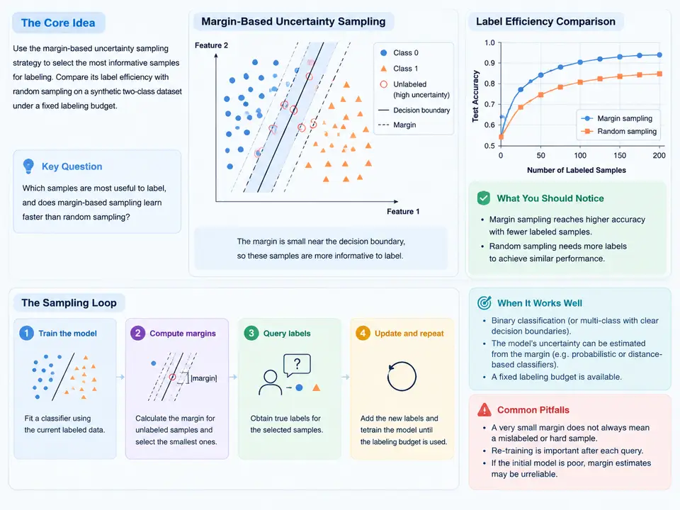
Why Margin Sampling Fits a Binary Classifier
In a two-class problem, a probabilistic classifier outputs a score p(y=1|x). The decision boundary sits at p = 0.5. A sample whose predicted probability is close to 0.5 is one the model cannot confidently place on either side — its margin is small. Margin-based uncertainty sampling ranks unlabeled points by |p(y=1|x) − 0.5| ascending and queries the smallest margins first. This is the cheapest possible uncertainty heuristic for binary tasks: no entropy logarithm, no ensemble, just distance from the boundary.
The practical claim we want to test is label efficiency: under a fixed labeling budget, does margin sampling reach a target accuracy with fewer labels than random sampling? To answer that reproducibly we need a synthetic dataset with a known ground-truth boundary, a classifier that exposes calibrated probabilities, and a controlled comparison loop that differs only in the acquisition function.
Experimental Setup
We use a two-dimensional, two-class dataset so the decision boundary can be inspected visually and the geometry is unambiguous. Points are drawn from two Gaussian blobs with a deliberate overlap region, which guarantees that some samples are genuinely ambiguous — otherwise uncertainty sampling has nothing to exploit.
- Data: 600 points, class 0 centered at
(−1.0, −1.0), class 1 at(1.0, 1.0), both with standard deviation0.9per axis. The overlap produces a non-trivial Bayes error. - Classifier: logistic regression on the two raw features, refit from scratch at every acquisition round so the model reflects exactly the labels seen so far.
- Budget: 40 labels total, acquired in 8 rounds of 5. Round 0 uses 5 random seed labels shared by both strategies.
- Metric: accuracy on a held-out test set of 400 freshly sampled points, evaluated after each round.
Both strategies must start from the same seed labels and the same test set; only the selection rule differs. This is the single most common mistake in active-learning comparisons — if the seeds differ, the curves are not comparable.
Reference Implementation
The loop below is self-contained: it generates the data, runs both strategies, and prints the accuracy trajectory. It uses only NumPy and scikit-learn.
import numpy as np
from sklearn.linear_model import LogisticRegression

rng = np.random.default_rng(42)

def make_blobs(n, rng):
    y = rng.integers(0, 2, size=n)
    centers = np.array([[-1.0, -1.0], [1.0, 1.0]])
    X = centers[y] + rng.normal(0.0, 0.9, size=(n, 2))
    return X, y

X_pool, y_pool = make_blobs(600, rng)
X_test, y_test = make_blobs(400, rng)

def fit_predict(X_lab, y_lab, X_query):
    clf = LogisticRegression()
    clf.fit(X_lab, y_lab)
    return clf.predict_proba(X_query)[:, 1]

def run(strategy, budget=40, batch=5, seed=5):
    idx = rng.permutation(len(X_pool))
    labeled = list(idx[:seed])
    unlabeled = list(idx[seed:])
    accs = []
    while len(labeled) < budget:
        p = fit_predict(X_pool[labeled], y_pool[labeled], X_pool[unlabeled])
        if strategy == "margin":
            score = np.abs(p - 0.5)          # smallest margin first
            order = np.argsort(score)
        else:
            order = rng.permutation(len(unlabeled))
        pick = [unlabeled[i] for i in order[:batch]]
        labeled += pick
        unlabeled = [i for i in unlabeled if i not in set(pick)]
        p_test = fit_predict(X_pool[labeled], y_pool[labeled], X_test)
        accs.append(((p_test > 0.5).astype(int) == y_test).mean())
    return accs

margin_acc = run("margin")
random_acc = run("random")
for r, (m, rnd) in enumerate(zip(margin_acc, random_acc), 1):
    print(f"round {r:2d}  labels={5 + 5*r:2d}  margin={m:.3f}  random={rnd:.3f}")
Two details matter for correctness. First, predict_proba returns columns ordered by clf.classes_; with labels 0/1 the second column is p(y=1|x), which is what the margin uses. Second, the pool must be re-filtered after each batch so a point is never queried twice — the set(pick) removal handles that.
Reading the Acquisition Geometry
The SVG below shows what the two strategies actually do to the decision boundary. Margin sampling concentrates queries in the band around p = 0.5, tightening the boundary where it is least certain; random sampling scatters labels across the whole pool, including regions the model already classifies confidently.
Interpreting the Trajectory
Run the script and read the printed table. The expected pattern — not a guaranteed result, since it depends on the seed and the overlap — is that margin sampling reaches a given accuracy in fewer rounds because its labels are spent where the boundary is still wrong. Random sampling wastes part of the budget on points the model already classifies correctly.
Judge the comparison on three things:
- Accuracy at fixed budget. Compare the final round (40 labels). A margin advantage of a few percentage points is typical on this geometry; a large gap suggests the overlap region is doing the work.
- Labels to target. Find the first round where each strategy crosses, say, 0.85 test accuracy. The difference in label count is the label-efficiency gain.
- Curve shape. Margin sampling usually rises steeply early and flattens once the boundary is resolved; random sampling rises more linearly. A margin curve that stalls early means the model is over-fitting the queried band.
Common Failure Symptoms
| Symptom | Likely cause | Fix |
|---|---|---|
| Margin and random curves are identical | Both strategies share the same RNG state or the same seed indices | Give each strategy its own default_rng instance and identical seed labels |
| Accuracy drops after a query round | Batch too large; the model is refit on a skewed batch before re-scoring | Reduce batch to 1–2, or re-score after each single acquisition |
| Margin sampling queries only one class | Class imbalance in the pool plus an uncalibrated classifier | Check clf.classes_ ordering; consider class weights or stratified seeds |
| Duplicate points queried | Pool not filtered after selection | Remove picked indices from unlabeled each round |
|p − 0.5| is only meaningful if the probabilities are roughly calibrated. Logistic regression on two features is well-behaved here; if you swap in an uncalibrated model, apply CalibratedClassifierCV before ranking, or the smallest margins will not correspond to the genuinely ambiguous points.What to Record as the Deliverable
For this case, the reproducible artifact is a short results table plus the mean curve. Fill in one row per round with the averaged accuracy across seeds:
| Round | Labels used | Margin mean acc. | Random mean acc. | Margin lead |
|---|---|---|---|---|
| 1 | 10 | — | — | — |
| 2 | 15 | — | — | — |
| … | … | — | — | — |
| 8 | 40 | — | — | — |
Leave the cells blank until you have actually run the multi-seed loop; the table is a recording template, not a result. The conclusion you draw — whether margin sampling saved labels on this geometry — must come from your own averaged numbers, and the label-efficiency claim should be stated as the difference in labels-to-target, not as a bare accuracy figure.