1. LS-DYNA simulation results landscape
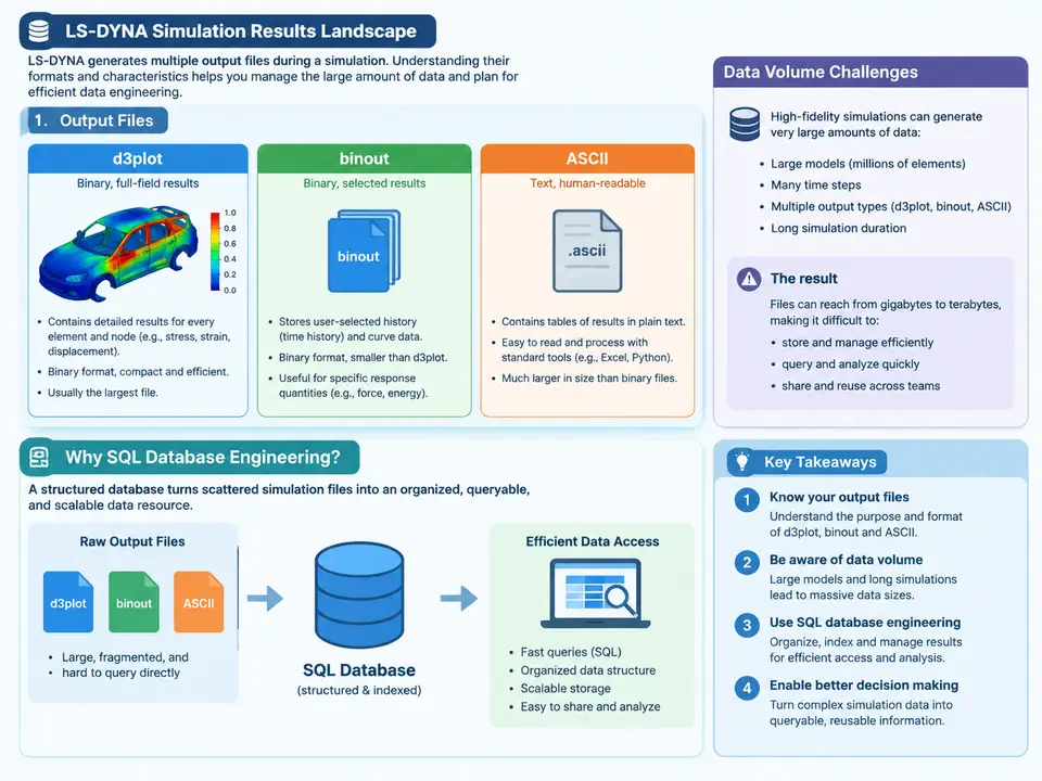
LS-DYNA is an explicit finite element solver used for crashworthiness, blast, drop, impact, and metal-forming analysis. A single run of a realistic vehicle crash model can produce dozens of output files in several distinct formats, each serving a different purpose and each carrying a different cost in storage and post-processing effort. Before any database schema can be designed, the engineer must understand what these files contain, how they are structured, and why they resist naive storage strategies. This chapter maps that landscape and establishes why SQL database engineering becomes necessary once simulation output moves beyond a handful of runs.
The Three Output Families
LS-DYNA writes results through three principal channels, controlled by keywords in the input deck. Each channel has a characteristic structure, access pattern, and volume profile.
d3plot — the binary state database. The *DATABASE_BINARY_D3PLOT keyword controls this family. The solver writes a sequence of binary state files (d3plot, d3plot01, d3plot02, …) at intervals defined by DT (simulation time between states) or NPLTC (cycle interval). Each state contains the full mesh geometry, nodal coordinates, nodal velocities and accelerations, element stresses and strains, and shell/beam section forces. For a 2-million-element model with 100 states, the d3plot family alone can exceed 50 GB. The files are read sequentially by LS-PrePost and by the d3plot reader libraries; they are not random-access in any practical sense.
binout — the time-history database. The *DATABASE_BINARY_BINOUT keyword (and its companion *DATABASE_HISTORY_* cards) produces a single binary file, binout, containing channelized time histories: nodal accelerations at selected nodes, interface forces from *CONTACT definitions, rigid-wall forces, section forces, and energy summaries. The binout format is a directory-structured binary container: a header indexes named channels, and each channel stores a time vector plus one or more data arrays. Tools such as lasso and the LS-DYNA Python reader expose these channels by name, for example binout/glstat for global energy or binout/nodout for nodal time histories.
ASCII — the human-readable reports. Keywords such as *DATABASE_ASCII_GLSTAT, *DATABASE_ASCII_MATSUM, *DATABASE_ASCII_RCFORC, and *DATABASE_ASCII_SLEOUT produce plain-text files (glstat, matsum, rcforc, sleout). These are small — typically kilobytes to a few megabytes — and contain tabular columns: time, kinetic energy, internal energy, hourglass energy, contact energy, and so on. They are the first files an engineer inspects when a run terminates abnormally or when energy balance must be verified.
Why Volume Alone Is Not the Real Problem
The raw size of a d3plot family is the obvious challenge, but it is not the one that most often defeats engineering teams. The harder problem is query shape. Consider the questions engineers actually ask across a design study of 40 crash simulations: Which run produced the highest peak acceleration at the driver seat rail? Which configuration had hourglass energy exceeding 5% of internal energy at any state? For the runs that passed the intrusion criterion, what was the correlation between B-pillar section force and door intrusion? These are cross-run, cross-channel, attribute-filtered queries. They cannot be answered by opening files one at a time in LS-PrePost, and they cannot be answered by a filesystem directory listing.
A second structural problem is heterogeneity. The same physical quantity appears in different channels with different names and different sampling. Nodal acceleration at a given node may exist in binout/nodout at every solver cycle, in d3plot at every output state, and in an ASCII nodout file at a coarser interval. Cross-referencing these requires a canonical identity for the node, the run, and the time base — precisely the kind of identity management a relational schema provides.
A third problem is provenance and reproducibility. A results directory named run_042_final_v3 carries no reliable record of which input deck, which solver version, which material parameter set, and which mesh revision produced it. When a result is challenged six months later, the file tree is not an audit trail.
What SQL Database Engineering Contributes
SQL database engineering addresses these problems by separating the storage layer from the query layer. The large binary payloads — d3plot states, full binout channels — remain in a file store or object store, addressed by a stable key. The metadata and the analytically relevant scalars move into relational tables: one row per run, one row per output channel, one row per extracted time-history sample or per state-level summary metric. Once that separation exists, the cross-run queries above become ordinary SQL joins and aggregates.
The design principle is selective extraction, not wholesale ingestion. A 50 GB d3plot family should not be loaded into a database row by row; instead, the engineer defines which scalars matter for the study — peak values, times of peak, integrals, pass/fail flags against criteria — and extracts those into narrow tables. The full binary remains available for detailed replay when a specific run needs visual inspection. This keeps the database in the gigabyte range while the file store holds the terabytes.
A Concrete Illustration of the Extraction Boundary
Suppose a study tracks occupant safety across 40 frontal impact runs. The analytically decisive quantities are: peak resultant acceleration at three specified nodes, peak intrusion at four section locations, maximum hourglass-to-internal energy ratio, and total run wall-clock time. Each of these is a scalar or a small fixed-length vector per run. Extracting them yields a table of roughly 40 rows by 10 columns — a few kilobytes — that answers every cross-run question in the study. The corresponding d3plot families total perhaps 2 TB and are consulted only when a specific run's animation must be reviewed.
The extraction itself is a defined procedure, not an ad-hoc script. For each run, the engineer reads the relevant binout channels by name, computes the peak and its time index, reads the ASCII glstat for the energy ratio, and writes one row. The procedure must record the channel name, the node or section ID, the sampling interval, and the extraction script version alongside the values, so that a later re-extraction can be reconciled. This provenance discipline is what distinguishes a results database from a spreadsheet of numbers.
Scope of the Engineering Discipline
The remainder of this course builds the discipline in layers: schema design for runs, channels, and extracted metrics; ingestion pipelines that parse binout and ASCII reliably; indexing and partitioning strategies for time-series tables; validation queries that catch extraction errors before they propagate into design decisions; and integration patterns that keep the database synchronized with the file store as new runs arrive. The starting point, established in this chapter, is a clear mental model of what LS-DYNA produces and which parts of that output belong in a relational store.
| Output family | Controlling keyword | Typical content | Access pattern | Database role |
|---|---|---|---|---|
| d3plot | *DATABASE_BINARY_D3PLOT |
Full mesh, nodal and element state per output time | Sequential state scan | File store; only extracted scalars enter SQL |
| binout | *DATABASE_BINARY_BINOUT |
Named time-history channels (nodout, rcforc, glstat, …) | Channel lookup by name | Primary source for time-series extraction |
| ASCII | *DATABASE_ASCII_* |
Column-oriented text tables (glstat, matsum, sleout) | Line-by-line parse | Direct load into summary tables |
The engineering conclusion is straightforward: LS-DYNA output is rich, heterogeneous, and large, and its value across a design study is realized only when the analytically relevant subset is lifted into a queryable, provenance-tracked relational structure. That lift is the subject of the chapters that follow.