1. CAE injury extraction fundamentals
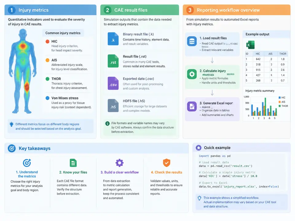
Crashworthiness and occupant-safety CAE post-processing is a data-reduction problem before it is a reporting problem. A single full-vehicle frontal impact run may produce hundreds of thousands of time steps across dozens of output requests, yet the deliverable that engineering management and certification teams actually consume is a compact table of peak values, time-of-peak, and pass/fail status against regulatory or internal targets. The purpose of this chapter is to establish the vocabulary and the pipeline that the rest of the course automates: what injury metrics mean physically, where they live inside a CAE result file, and how a repeatable extraction-to-Excel workflow is structured.
Injury metrics and what they physically represent
Injury criteria are biomechanical correlates of tissue damage, reduced to scalar functions of measured acceleration, force, moment, or deflection. In occupant simulation the most common family is head injury assessment. The Head Injury Criterion (HIC) integrates the resultant translational acceleration at the head center of gravity over a 36 ms window:
HIC = max over (t1, t2) of [ (t2 - t1) * ( (1/(t2-t1)) * ∫ a_r(t) dt )^2.5 ]
subject to: t2 - t1 ≤ 36 ms,  a_r in g
Two implementation details matter enormously in practice. First, a_r is the resultant of the three translational channels, so the sign convention of the accelerometer axes is irrelevant to HIC but critical to any directional metric. Second, the integration window is a sliding search, not a fixed interval; a naive implementation that evaluates only the full 36 ms window will systematically under-report HIC when the true peak occurs in a shorter sub-window. The same sliding-window logic applies to the 15 ms variant HIC15 used in some regulations.
Chest injury is typically expressed as chest deflection (in mm) or as the Chest Injury Index / viscous criterion V*C, which couples compression and compression rate. Neck injury uses Nij, a dimensionless combination of axial force and bending moment normalized by injury reference values (Nij = Fz/Fint + My/Mint). Femur force, tibia index, and pelvis acceleration round out the lower-extremity set. Each metric has a defined normalization, a defined filter, and a defined evaluation window — and the extraction script must reproduce all three exactly, or the numbers will not match the certification report.
Where the data lives: CAE result file structure
Regardless of solver, a transient occupant result file is organized as a set of output blocks, each keyed by a node or element ID and carrying a time-history array. In LS-DYNA the relevant containers are nodout (nodal displacements, velocities, accelerations) and elout; in PAM-CRASH and Radioss the equivalents are time-history and animation files. The practical consequence is that extraction is an ID lookup plus channel selection problem: you must know which node ID corresponds to the head CG, which to the chest accelerometer location, and which channel index within the block holds the quantity you want.
A robust extraction layer therefore keeps a small mapping table separate from the solver-specific reader. The table below shows the kind of mapping that a real project maintains; the IDs are illustrative.
| Metric | Source block | Node / element ID | Channel | Filter | Target |
|---|---|---|---|---|---|
| HIC36 | nodout | 900112 (head CG) | ax, ay, az | CFC 600 | ≤ 700 |
| Chest deflection | nodout | 900340 / 900341 | relative Y | CFC 180 | ≤ 63 mm |
| Nij | nodout | 900201 (neck top) | Fz, My | CFC 600 | ≤ 1.0 |
| Femur force | nodout | 900510 (left knee) | Fz | CFC 600 | ≤ 10 kN |
Two failure modes dominate this stage. The first is ID drift: when the model is re-meshed or the dummy is repositioned, node IDs change and a hard-coded script silently reads the wrong channel, producing plausible but wrong numbers. The second is time-base mismatch: solver output may be written at a coarser interval than the integration step, and resampling without interpolation introduces step artifacts into the HIC integral. Both are addressed by validating extracted curves against a known reference run before trusting the batch output.
The extraction-to-report workflow
The end-to-end pipeline has five stages, and the boundaries between them are what make the automation maintainable. The diagram below shows the data flow and the artifacts exchanged at each boundary.
The first stage is deliberately dumb: it opens the result file and exposes time-history arrays by node ID, with no knowledge of injury criteria. The second stage is pure configuration — the mapping table shown earlier. The third stage is where the biomechanics lives: filtering, resultant computation, sliding-window search, and unit normalization. The fourth stage compares each computed value against its target and records the margin. The fifth stage writes the workbook. Keeping these stages separate means a new load case requires only a new mapping row and a new input path, not a code change.
A minimal worked example
Consider a head acceleration channel sampled at 10 kHz over 120 ms, with a peak resultant of 85 g sustained for roughly 3 ms. A correct HIC36 evaluation slides a 36 ms window across the record, computes the mean resultant acceleration within each candidate window, raises it to the 2.5 power, multiplies by the window duration, and takes the maximum. For a short, high-amplitude pulse the maximizing window is typically much shorter than 36 ms — often 5–15 ms — which is exactly why the sliding search is mandatory. The output row would carry the peak HIC value, the start and end times of the maximizing window, and a pass/fail flag against the 700 target. If the same channel is read without the CFC 600 filter, the peak will be higher and the reported HIC will not reproduce the sled-test correlation; that discrepancy is the diagnostic signal that the filter stage was skipped.
With this foundation — metric definitions, file structure, and the five-stage pipeline — the remaining chapters can treat each stage as an engineering task in its own right: parsing solver output reliably, implementing the criteria correctly, and generating a workbook that a reviewer can audit without re-running the solver.