1. Course introduction
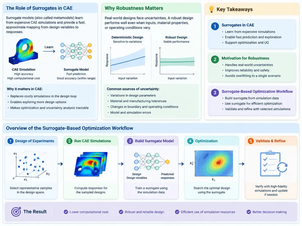
Computer-aided engineering (CAE) has become the backbone of modern product development. A single high-fidelity finite element analysis (FEA) or computational fluid dynamics (CFD) run can take minutes to days, and a design optimization study may require thousands of such runs. When each evaluation costs hours, the optimizer spends most of its budget waiting on the solver rather than exploring the design space. This is the central bottleneck that machine learning surrogates are designed to remove.
A surrogate model — also called a metamodel or response surface — is a cheap mathematical approximation of an expensive simulation. It is trained on a limited set of high-fidelity samples and then evaluated in microseconds. The surrogate does not replace the physics; it compresses the input–output behavior of the physics into a form that can be queried at scale. The practical consequence is that an optimization loop that once required 5,000 solver calls can often be completed with 150–300 training samples plus tens of thousands of surrogate evaluations.
Why Surrogates Matter in CAE
Consider a representative engineering scenario: a bracket must be lightweight while keeping peak von Mises stress below a yield limit. Each nonlinear static FEA run with a fine mesh takes roughly 12 minutes on 16 cores. A genetic algorithm with a population of 40 over 60 generations needs 2,400 evaluations — about 480 core-hours, or three weeks of wall-clock time on a single workstation. With a surrogate trained on 200 Latin hypercube samples (40 core-hours), the same optimization completes overnight, and the final candidate designs are then verified with full FEA.
Surrogates deliver value in four recurring ways:
- Cost compression. Replacing solver calls with model inference reduces evaluation cost by three to five orders of magnitude.
- Noise smoothing. Mesh-induced numerical noise in stress or drag outputs can mislead gradient-based optimizers; a fitted surrogate provides a smooth, differentiable response surface.
- Design-space exploration. Surrogates enable sensitivity screening, what-if analysis, and visualization of response landscapes before committing to expensive runs.
- Real-time use. Once trained, a surrogate can be embedded in dashboards, digital twins, or control loops where simulation latency is unacceptable.
The Motivation for Robustness
Deterministic optimization pushes designs to constraint boundaries: stress exactly at yield, frequency exactly at the limit. Such designs are optimal on paper but fragile in reality. Manufacturing tolerances shift wall thickness by ±0.2 mm; material properties vary by 5–10%; operating loads fluctuate. A design sitting on the constraint boundary will violate it under any of these perturbations.
Robust optimization explicitly accounts for this. Instead of optimizing the nominal response, it optimizes a statistical measure — typically the mean plus a weighted standard deviation, or the probability of constraint satisfaction. Formally, a robust objective can be written as:
minimize   J = μ(f(x, ξ)) + k · σ(f(x, ξ))
subject to P(g(x, ξ) ≤ 0) ≥ 1 − α
where      x = design variables, ξ = uncertain parameters
           μ, σ = mean and standard deviation of the response
           k = robustness weight, α = allowable failure probability
Evaluating μ and σ requires propagating uncertainty through the simulation — Monte Carlo sampling, for instance, with 1,000 realizations per design. Doing this with full FEA is computationally prohibitive. This is precisely where surrogates become essential: the surrogate is evaluated thousands of times per design to estimate the statistics, making robust optimization tractable.
Overview of the Surrogate-Based Optimization Workflow
The workflow below is the backbone of the entire course. Each stage introduces decisions that materially affect the final result, and later chapters examine each in depth.
Two features of this workflow deserve emphasis at the outset. First, the adaptive infill loop (dashed path from stage 7 back to stage 3) is what distinguishes modern surrogate-based optimization from classical response-surface methods. Rather than training once on a fixed sample set, the algorithm iteratively adds high-fidelity samples where the surrogate is uncertain or where the optimum is likely to lie. This is the core idea behind efficient global optimization (EGO) and Bayesian optimization. Second, verification with the full solver is non-negotiable. A surrogate is a hypothesis about the physics; the final design must be confirmed against the actual simulation before it is accepted.
What This Course Covers
The course is organized around the workflow above, moving from foundations to advanced robust methods:
- Surrogate foundations. Sampling strategies (Latin hypercube, Sobol sequences), model families (Gaussian process/Kriging, radial basis functions, polynomial response surfaces, neural network surrogates), and accuracy assessment via cross-validation and error metrics such as R² and normalized RMSE.
- Adaptive sampling and optimization. Expected improvement, probability of improvement, and lower confidence bound acquisition functions; convergence criteria and stopping rules.
- Uncertainty quantification. Propagating manufacturing and material uncertainty through the surrogate; Monte Carlo, polynomial chaos, and moment-based methods.
- Robust and reliability-based optimization. Formulating μ + k·σ objectives, chance constraints, and reliability indices; handling the trade-off between performance and robustness.
- Engineering practice. Solver integration, data pipelines, surrogate versioning, and validation protocols for industrial deployment.
A First Worked Example
To make the workflow concrete, consider a simplified cantilever beam design. The design variable is the cross-section height h ∈ [20, 60] mm, with width fixed at 30 mm and length 500 mm. The load F is uncertain, modeled as a normal distribution with mean 2,000 N and standard deviation 200 N. The constraint is that maximum bending stress must not exceed 150 MPa.
The deterministic optimum pushes h to its lower bound, where nominal stress equals 150 MPa. But with F varying by ±10%, roughly half of all realizations exceed the limit. A robust formulation minimizes mass subject to P(σ ≤ 150 MPa) ≥ 0.99. Running 1,000 Monte Carlo samples per candidate on a trained Kriging surrogate (trained on 80 FEA samples) yields a robust optimum at h ≈ 34 mm — heavier than the deterministic design but with a 99% probability of meeting the stress constraint. The final candidate is then verified with full FEA, confirming the surrogate prediction within 2%.
With this foundation in place, the following chapters build each stage of the workflow in detail, beginning with the sampling and surrogate-modeling techniques that make everything else possible.