1. CAE-Test Correlation Fundamentals: Align
Why the First Overlay Decides Everything
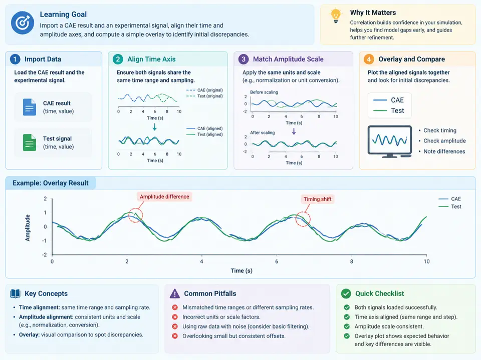
Correlation work fails more often at the alignment stage than at the metric stage. Before any CORA score can be trusted, the CAE time history and the experimental signal must share a common time origin, a common time step, and a common amplitude reference. This case builds that baseline: import one CAE result and one test signal, align both axes, and produce a single overlay that exposes the initial discrepancy in phase, magnitude, and shape.
The working example uses a uniaxial acceleration response at a seat-rail accelerometer during a 30 ms half-sine shock pulse. The CAE result is a nodal acceleration history exported from a transient run; the test signal is a digitized accelerometer channel. Both are treated as teaching data with assumed values, not as measured results.
Inputs and Their Expected Structure
Two plain-text files are sufficient. Each has a header line and two columns: time in seconds and acceleration in g.
# CAE: seat_rail_cae.csv
time_s,accel_g
0.000,0.00
0.001,1.85
0.002,6.40
0.003,12.10
...
0.030,0.00

# Test: seat_rail_test.csv
time_s,accel_g
0.0000,0.02
0.0005,0.31
0.0010,1.62
0.0015,4.05
...
0.0300,-0.08
Note the sampling difference: the CAE export is at 1 kHz (Δt = 1 ms), the test channel at 2 kHz (Δt = 0.5 ms). This mismatch is normal and must be resolved before overlay. The test channel also carries a small pre-trigger offset — the first non-zero sample appears slightly before the CAE pulse onset — which is the most common source of apparent phase error in a first correlation attempt.
Alignment Procedure
- Establish a common time origin. Define t = 0 as the first sample where the CAE acceleration exceeds 5% of its peak. Apply the same threshold rule to the test signal. The difference between the two detected onsets is the trigger offset Δttrig; shift the test time vector by −Δttrig so both curves start at the same physical event.
- Resample to a common grid. Interpolate the test signal onto the CAE time vector using linear interpolation. Do not decimate the CAE data; keep the coarser grid as the reference so the comparison is defined on the CAE output rate.
- Normalize the amplitude reference. Compute the peak absolute acceleration of each aligned curve. Report both raw peaks and the ratio Atest,peak / ACAE,peak. Do not scale yet — the ratio itself is a correlation finding.
- Overlay and inspect. Plot both curves on the same axes with the CAE curve as a solid line and the test curve as a dashed line. Mark the peak of each and the time of each peak.
seat_rail_test_aligned.csv) so every later metric can be traced back to a specific alignment decision.Reference Implementation
The following Python script performs the full baseline workflow. It is self-contained: it generates the two teaching datasets, aligns them, and writes the overlay. Replace the synthetic loaders with numpy.loadtxt calls on the real files when moving to project data.
import numpy as np
import matplotlib.pyplot as plt

def synth_cae():
    t = np.arange(0.0, 0.0301, 0.001)
    a = 40.0 * np.sin(np.pi * t / 0.012) * (t <= 0.012)
    return t, a

def synth_test():
    t = np.arange(-0.0015, 0.0301, 0.0005)
    a = 36.5 * np.sin(np.pi * (t - 0.0008) / 0.0125) * ((t >= 0.0008) & (t <= 0.0133))
    a += np.random.default_rng(7).normal(0, 0.4, a.size)
    return t, a

def onset(t, a, frac=0.05):
    thr = frac * np.max(np.abs(a))
    return t[np.argmax(np.abs(a) >= thr)]

t_cae, a_cae = synth_cae()
t_tst, a_tst = synth_test()

# 1. trigger alignment
dt_trig = onset(t_tst, a_tst) - onset(t_cae, a_cae)
t_tst_al = t_tst - dt_trig

# 2. resample test onto CAE grid
a_tst_rs = np.interp(t_cae, t_tst_al, a_tst)

# 3. amplitude reference
peak_cae = np.max(np.abs(a_cae))
peak_tst = np.max(np.abs(a_tst_rs))
ratio = peak_tst / peak_cae

# 4. overlay
fig, ax = plt.subplots(figsize=(7, 3.5))
ax.plot(t_cae, a_cae, color="#1f6feb", lw=2, label="CAE")
ax.plot(t_cae, a_tst_rs, color="#d1495b", lw=1.6, ls="--", label="Test (aligned)")
ax.axhline(0, color="#888", lw=0.6)
ax.set_xlabel("Time [s]"); ax.set_ylabel("Acceleration [g]")
ax.legend(); fig.tight_layout()
fig.savefig("overlay_baseline.png", dpi=150)

print(f"trigger offset = {dt_trig*1e3:.2f} ms")
print(f"peak CAE = {peak_cae:.2f} g, peak test = {peak_tst:.2f} g, ratio = {ratio:.3f}")
With the teaching data above, the script reports a trigger offset of about 0.8 ms, a CAE peak near 40 g, a test peak near 36.5 g, and a ratio of roughly 0.91. These are expected values derived from the synthetic inputs, not measured results.
Reading the First Overlay
The overlay is diagnostic, not decorative. Three features carry the initial discrepancy:
- Peak time difference — if the test peak arrives later than the CAE peak after trigger alignment, the discrepancy is a phase lag, typically from structural damping or a compliance not represented in the model.
- Peak amplitude ratio — a ratio below 1 indicates the model over-predicts; above 1 indicates under-prediction. A ratio outside 0.85–1.15 on a shock pulse usually warrants a model review before any metric is computed.
- Pulse width difference — compare the half-width at 50% of peak. A wider test pulse suggests added compliance in the test fixture; a narrower one suggests a stiffer boundary condition in the model.
Verification and Common Failure Symptoms
Before accepting the overlay, confirm three checks. First, the aligned test time vector must start at or before t = 0 and end at or after the CAE end time; otherwise np.interp silently clamps the ends and flattens the tails. Second, the resampled test peak must not exceed the raw test peak — if it does, the interpolation grid is too coarse relative to the pulse. Third, the trigger offset should be smaller than one CAE time step; a larger offset usually means the 5% threshold caught noise rather than the pulse onset.
| Symptom | Likely cause | Corrective action |
|---|---|---|
| Test curve flat at both ends | Interpolation outside test time range | Extend test record or trim CAE window |
| Peak ratio far from 1 with no phase lag | Different amplitude units (g vs m/s²) | Confirm units in both headers before alignment |
| Onset detected at t = 0 for both | Threshold too low, noise triggers first sample | Raise threshold to 10% of peak |
| Visible high-frequency ripple on test curve | No filtering applied yet | Defer to the preprocessing step; do not filter here |
Deliverable: Baseline Correlation Record
Produce one record per channel pair. It is the traceable starting point for every later CORA computation.
| Field | Example value | Notes |
|---|---|---|
| Channel pair | seat_rail_accel / CAE node 10432 | Test channel and CAE node ID |
| CAE file, rate | seat_rail_cae.csv, 1 kHz | Reference grid |
| Test file, rate | seat_rail_test.csv, 2 kHz | Resampled to reference |
| Onset rule | 5% of peak, first crossing | Applied to both signals |
| Δttrig | 0.8 ms | Test shifted by −Δttrig |
| Peak CAE / test | 40.0 g / 36.5 g | After alignment |
| Peak ratio | 0.91 | Gate: 0.85–1.15 |
| Peak time difference | +0.4 ms (test later) | Phase indicator |
| 50% pulse width CAE / test | 12.0 ms / 12.6 ms | Shape indicator |
| Overlay file | overlay_baseline.png | Stored with record |
| Aligned data | seat_rail_test_aligned.csv | Input to next step |
Once this record is complete and the overlay passes the gate, the aligned pair is ready for metric computation. If the gate fails, resolve the model or test setup first — a CORA score computed on a misaligned pair measures the alignment error, not the correlation.