1. CAE-driven design optimization landscape
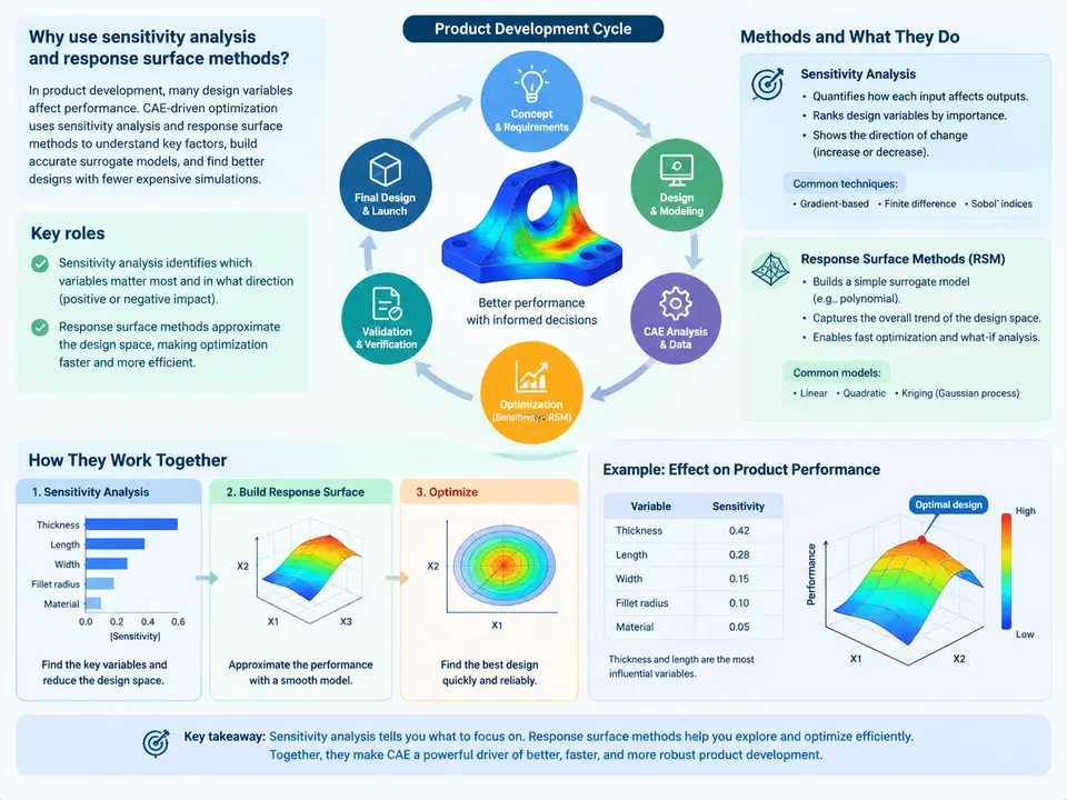
Modern product development rarely has the luxury of iterating on physical prototypes alone. A single full-vehicle crash validation, a thermal soak test on an electronics enclosure, or a fatigue qualification of a turbine blade can consume weeks and six-figure budgets. Computer-aided engineering (CAE) shifts much of that learning loop into simulation, but simulation by itself does not optimize anything — it only reports what a given design does. The discipline that turns simulation into design decisions is design optimization, and its two workhorses are sensitivity analysis and response surface methods (RSM).
This chapter frames where those two techniques sit in a real development cycle, what each contributes, and how they chain together. The goal is not to master the mathematics yet, but to build an accurate mental model of the optimization landscape so that later chapters on DOE, metamodeling, and multi-objective trade studies have a place to attach.
The three layers of a CAE optimization workflow
A useful way to organize the field is a three-layer stack. At the bottom sits the simulation model: the finite element mesh, boundary conditions, material laws, and solver settings that produce a response such as maximum von Mises stress, first natural frequency, or pressure drop. Above it sits the design space: the set of input variables — plate thickness, fillet radius, rib spacing, material grade — each with a baseline value and a permissible range. At the top sits the optimization strategy: the algorithm or surrogate that decides which designs to evaluate and how to move toward better ones.
Sensitivity analysis and RSM are the two bridges between the design space and the optimization strategy. Sensitivity analysis asks a local question: if I perturb this variable by a small amount, how much does the response change? RSM asks a global question: can I approximate the entire response over the design space with a cheap mathematical function? The first is a derivative; the second is a map. Both are needed because a single CAE solve is expensive, and an optimizer may want hundreds or thousands of evaluations.
What sensitivity analysis actually delivers
In practice, sensitivity analysis is the first thing an engineer runs after a baseline solve, because it answers the question every design review starts with: which knobs matter? The most common form is the normalized sensitivity coefficient, often written as
S_i = (∂y / ∂x_i) · (x_i / y)where y is the response and x_i is the i-th design variable. Normalizing by x_i / y makes coefficients dimensionless, so a thickness sensitivity and a fillet-radius sensitivity can be compared on the same scale. A coefficient of 0.8 means a 1% change in that variable produces roughly a 0.8% change in the response; a coefficient near 0.02 means the variable is nearly irrelevant and can be frozen to reduce the design space.
For a bracket example, suppose the baseline is t = 4 mm, r = 6 mm, with baseline σ_max = 180 MPa and f₁ = 240 Hz. A finite-difference run with a 5% perturbation might return:
| Variable | Baseline | Perturbation | Δσ_max | Normalized S (stress) | Normalized S (f₁) |
|---|---|---|---|---|---|
| Plate thickness t | 4.0 mm | +5% → 4.2 mm | −9.4 MPa | −1.04 | +0.31 |
| Fillet radius r | 6.0 mm | +5% → 6.3 mm | −3.1 MPa | −0.34 | −0.05 |
| Rib spacing s | 40 mm | +5% → 42 mm | +0.6 MPa | +0.03 | −0.02 |
These numbers are illustrative, not measured, but the pattern is typical: thickness dominates stress, the fillet has a meaningful but secondary effect, and rib spacing is nearly inert for this load case. That single table already reshapes the optimization plan — freeze s, keep t and r as active variables, and expect the optimizer to push thickness down until the stress constraint binds.
Why response surfaces enter the picture
Sensitivity analysis tells you the slope at one point. It does not tell you where the optimum is, and it cannot handle a design space with strong curvature or variable interactions efficiently. That is the job of the response surface. The idea is to fit a cheap analytical function ŷ(x) to a set of sampled CAE runs, then let the optimizer explore ŷ at negligible cost. A second-order polynomial is the classic choice:
ŷ = β₀ + Σ βᵢxᵢ + Σ βᵢᵢxᵢ² + Σ βᵢⱼxᵢxⱼThe cross terms βᵢⱼxᵢxⱼ are what make RSM more than a Taylor expansion — they capture interaction, for example the fact that a thin plate with a large fillet behaves differently from a thin plate with a small one. For highly nonlinear responses, Kriging or radial basis functions replace the polynomial, but the workflow is the same: sample, fit, validate, optimize on the surrogate, then confirm the predicted optimum with a full CAE solve.
The sampling plan matters as much as the fit. A full factorial on five variables at three levels is 243 runs — often impractical at 15 minutes per solve. A Latin hypercube or D-optimal design can cover the same space with 30–50 runs, which is the practical range for most industrial studies. The surrogate's quality is judged by R², adjusted R², and — more importantly — by a hold-out or cross-validation error on points not used in the fit. A surrogate with R² = 0.98 but a 12% prediction error at the candidate optimum is not trustworthy; the confirmation run is what closes the loop.
How the pieces fit into the development cycle
In a concept phase, sensitivity analysis is used to prune the variable list and set realistic ranges before any optimization budget is committed. In detailed design, RSM supports trade studies: the surrogate is cheap enough to sweep thousands of combinations and produce a Pareto front of mass versus stiffness, letting the team choose a design point rather than accept whatever the optimizer returns. In validation, the confirmed optimum is re-solved with the full model, and the difference between surrogate prediction and CAE result is the surrogate error that must be reported alongside the design.
The rest of this course builds each layer in turn: design-of-experiments and sampling, sensitivity formulations and their numerical pitfalls, surrogate construction and validation, and finally multi-objective optimization and robustness. The landscape above is the map; the following chapters are the terrain.