1. Import and Standardize Injury Curves fro
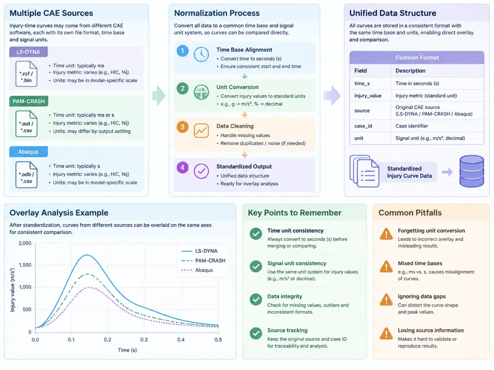
Why a unified injury-curve structure matters
Injury overlay analysis only becomes trustworthy when every curve entering the comparison shares the same time reference and the same physical units. LS-DYNA, PAM-CRASH, and Abaqus each export time histories in their own conventions: LS-DYNA ASCII curves typically carry time in milliseconds and accelerations in g or mm/ms²; PAM-CRASH result files often use seconds with accelerations in m/s²; Abaqus .csv/.dat exports may use seconds with rotations in radians and strains as dimensionless ratios. Loading them naively into one plot produces curves that are offset in time, scaled by 1000, or silently mixed between angular and linear quantities. The task here is to build a single loader that ingests all three formats and emits one normalized record per curve.
Target data structure
Define a canonical record before writing any parser. Every curve, regardless of source, is reduced to the following fields:
source— one of"lsdyna","pamcrash","abaqus".channel— the physical quantity, e.g."accel_x","strain_principal","force_z".t— 1-D array of time in seconds, strictly increasing.y— 1-D array of values in SI base units (m/s², Pa, N, dimensionless strain).meta— dict withoriginal_time_unit,original_value_unit,scale_applied, andn_samples.
Normalizing to SI at load time means downstream overlay code never has to remember which file used which unit. The meta block preserves provenance so a reviewer can audit any scaling decision.
Unit and time-base normalization rules
Apply a fixed conversion table. Time is always converted to seconds; values are converted to SI base units for the channel's physical dimension.
| Source | Typical time unit | Typical value unit | Conversion to canonical |
|---|---|---|---|
| LS-DYNA ASCII | ms | g (accel), mm (disp) | t × 1e-3; accel × 9.80665; disp × 1e-3 |
| PAM-CRASH | s | m/s², m | t × 1; accel × 1; disp × 1 |
| Abaqus CSV | s | m/s², strain (—) | t × 1; accel × 1; strain × 1 |
Two rules prevent the most common errors. First, never infer the time unit from the magnitude of the numbers — a 0.05 s event and a 50 ms event look identical after a careless read. Require the unit to be declared per file (via a sidecar or a header line) and record it in meta.original_time_unit. Second, convert acceleration to m/s² before any integration or filtering; converting after filtering changes the filter's effective cutoff.
Reference implementation
The loader below is self-contained: it defines the canonical record, three format-specific readers, and a dispatcher. It uses only the standard library plus numpy, and each reader is exercised by a small inline example so the behavior is verifiable without external files.
import csv
import numpy as np
from dataclasses import dataclass, field

G = 9.80665  # m/s^2 per g

@dataclass
class InjuryCurve:
    source: str
    channel: str
    t: np.ndarray
    y: np.ndarray
    meta: dict = field(default_factory=dict)

    def __post_init__(self):
        if self.t.ndim != 1 or self.y.ndim != 1 or self.t.size != self.y.size:
            raise ValueError("t and y must be 1-D and equal length")
        if np.any(np.diff(self.t) <= 0):
            raise ValueError("time vector must be strictly increasing")

def _finalize(source, channel, t, y, t_unit, y_unit, scale):
    t = np.asarray(t, dtype=float)
    y = np.asarray(y, dtype=float)
    return InjuryCurve(
        source=source, channel=channel, t=t, y=y,
        meta={"original_time_unit": t_unit,
              "original_value_unit": y_unit,
              "scale_applied": scale,
              "n_samples": int(t.size)},
    )

def load_lsdyna(path, channel, time_unit="ms", value_unit="g"):
    t_raw, y_raw = [], []
    with open(path) as fh:
        for row in csv.reader(fh, delimiter=","):
            if not row or row[0].startswith("#"):
                continue
            t_raw.append(float(row[0]))
            y_raw.append(float(row[1]))
    t_scale = {"ms": 1e-3, "s": 1.0}[time_unit]
    y_scale = {"g": G, "m/s2": 1.0, "mm": 1e-3, "m": 1.0}[value_unit]
    return _finalize("lsdyna", channel,
                     np.array(t_raw) * t_scale,
                     np.array(y_raw) * y_scale,
                     time_unit, value_unit, (t_scale, y_scale))

def load_pamcrash(path, channel, time_unit="s", value_unit="m/s2"):
    data = np.loadtxt(path, delimiter=",", comments="#")
    t_scale = {"s": 1.0, "ms": 1e-3}[time_unit]
    y_scale = {"m/s2": 1.0, "g": G}[value_unit]
    return _finalize("pamcrash", channel,
                     data[:, 0] * t_scale,
                     data[:, 1] * y_scale,
                     time_unit, value_unit, (t_scale, y_scale))

def load_abaqus(path, channel, time_unit="s", value_unit="m/s2"):
    data = np.genfromtxt(path, delimiter=",", names=True)
    t_scale = {"s": 1.0, "ms": 1e-3}[time_unit]
    y_scale = {"m/s2": 1.0, "g": G, "strain": 1.0}[value_unit]
    return _finalize("abaqus", channel,
                     data["time"] * t_scale,
                     data["value"] * y_scale,
                     time_unit, value_unit, (t_scale, y_scale))

LOADERS = {"lsdyna": load_lsdyna,
           "pamcrash": load_pamcrash,
           "abaqus": load_abaqus}

def load_curve(source, path, channel, **units):
    return LOADERS[source](path, channel, **units)
Each loader returns an InjuryCurve whose t is in seconds and whose y is in SI base units. The __post_init__ guard rejects non-monotonic time vectors, which is the most frequent defect in exported CAE curves (duplicate timestamps at restart points).
What the normalization pipeline looks like
The diagram below shows how three heterogeneous source files converge on one canonical record. It emphasizes the two independent conversions (time base and value unit) and the validation gate that every curve must pass before it is admitted to the overlay set.
Verification and failure symptoms
After loading, run three checks before any overlay. First, confirm t[0] == 0.0 and t[-1] matches the declared event duration in seconds — a value near 50 for a 50 ms LS-DYNA event means the time scale was not applied. Second, compare the peak of y against the source's reported peak; a factor of 9.81 indicates a missed g conversion, and a factor of 1000 indicates a missed millimetre conversion. Third, assert np.all(np.diff(curve.t) > 0); a ValueError from __post_init__ usually points to restart timestamps duplicated in the export, which should be de-duplicated at the source rather than silently averaged.
meta.scale_applied tuple lets you reconstruct the original number exactly, which is essential for injury-criterion traceability.Deliverable: normalization checklist
The following checklist can be applied to each incoming file before it is admitted to the overlay set.
| Check | Pass condition | Action on failure |
|---|---|---|
| Time unit declared | meta.original_time_unit in {ms, s} | Reject; request sidecar or header |
| Value unit declared | meta.original_value_unit matches channel dimension | Reject; do not guess from magnitude |
| Time monotonic | diff(t) > 0 everywhere | De-duplicate restart timestamps at source |
| Lengths aligned | t.size == y.size | Reject; truncated export |
| Peak sanity | Peak within 1% of source-reported peak | Re-check scale tuple in meta |
| Start time | t[0] == 0.0 | Shift by t[0] and record offset |
Once every curve passes these checks, the overlay stage can assume a common time origin and consistent SI units, and the remaining work — resampling onto a shared time vector — becomes a purely numerical problem rather than a data-cleaning one.