1. CAE simulation data landscape
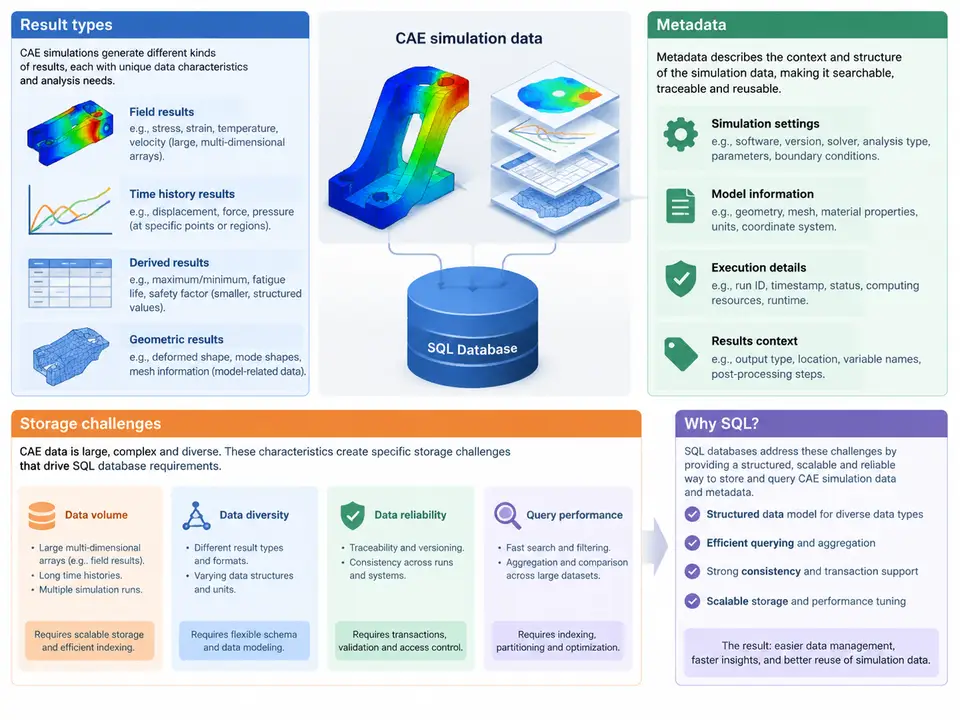
Computer-aided engineering (CAE) simulation produces data that is fundamentally different from the transactional records most database designers are trained on. A single explicit dynamic run may emit hundreds of time steps, each containing nodal displacements, element stresses, contact forces, and energy histories across millions of degrees of freedom. Before we can design a schema, we must understand what that data actually looks like, what describes it, and why naive storage strategies collapse under its weight. This chapter maps the CAE data landscape and derives the concrete requirements that will shape every table, index, and query in the rest of the course.
Result types: what a solver actually writes
CAE results fall into a small number of structural families, and each family has different cardinality and access patterns. Field results are the dominant category: scalar or vector quantities defined per node or per element, sampled at discrete time or load steps. Typical examples include nodal displacement (three components per node), element von Mises stress (one scalar per element or per integration point), and temperature fields. History results are time series attached to a small set of monitored entities — a single node's acceleration, a contact pair's normal force, or a rigid body's kinetic energy. Modal results add an eigenvalue dimension: each mode has a frequency and a mode shape that is itself a field. Scalar summaries — maximum stress, total mass, factor of safety — are low-cardinality aggregates that analysts query constantly.
The critical observation is that field results are sparse in meaning but dense in storage. A displacement field at one time step for a 2-million-node mesh is 6 million floating-point values. Multiply by 500 time steps and you have 3 billion values for one load case. History results, by contrast, may be only a few thousand rows. A schema that treats both identically will either waste enormous space or lose the ability to query efficiently.
Metadata: the context that makes results interpretable
A raw array of floats is worthless without the metadata that anchors it. In practice, every result set carries several metadata layers that must be modeled explicitly:
- Provenance — solver name and version, input deck hash, run timestamp, host, and user. This is what lets you answer "which results came from the model before the mesh was refined?"
- Model identity — mesh ID, node and element counts, coordinate system, units. Unit mismatches (mm vs. m, MPa vs. Pa) are a classic source of silent errors and must be stored, not assumed.
- Load case and step definition — load case name, step index, physical time or frequency, and the analysis type (static, transient, modal, explicit).
- Field descriptors — quantity name, component count, location (nodal vs. elemental vs. integration point), and tensor order.
Metadata is small but queried far more often than the bulk data. Analysts filter by load case, compare runs by input deck hash, and join results to mesh topology. This asymmetry — tiny, hot metadata versus huge, cold field data — is the single most important driver of the physical schema.
Storage challenges that force SQL design decisions
Three pressures dominate. First, volume and write throughput: a transient run can write gigabytes in minutes, and the database must ingest this without per-row overhead that would make a 3-billion-row insert take days. Second, query selectivity: the common analytical query is "give me the maximum von Mises stress over all elements at step 120 for load case LC3," which touches a narrow slice of a huge table. Without the right partitioning and indexing, this becomes a full scan. Third, heterogeneity: scalar, vector, and tensor fields coexist, and a rigid one-table-per-quantity design explodes into dozens of near-identical tables.
The figure below summarizes how these result families, their metadata, and the resulting storage pressures relate to one another — and where SQL design choices intervene.
From landscape to requirements
The landscape above translates directly into a set of non-negotiable database requirements. Separation of metadata and bulk data is the first: metadata tables stay small, normalized, and heavily indexed, while field values live in partitioned fact tables keyed by run, load case, and step. Partitioning by run and step keeps individual partitions manageable and lets the query planner prune irrelevant data. Composite indexes on the filter columns that analysts actually use — load case, step index, location — turn the representative query into a range scan. Explicit unit and coordinate-system columns prevent the silent errors that plague file-based workflows. And a stable mesh identity allows results from different runs to be compared and joined without ambiguity.
Consider a concrete example. A transient crash simulation writes 400 steps for a 1.2-million-element mesh, storing von Mises stress per element. That is 480 million rows in the field table. If the table is partitioned by run_id and sub-partitioned by step_index ranges, the query for step 120 of run 7 touches one partition of roughly 1.2 million rows. With a composite index on (load_case, step_index, location), the planner performs an index range scan and aggregates only the matching rows. The same query against an unpartitioned, unindexed table would scan 480 million rows — a difference of two to three orders of magnitude in latency. This is not a theoretical concern; it is the difference between an interactive dashboard and a batch job that runs overnight.
What this means for the schema you will build
Every subsequent chapter builds on the model established here. The result families determine table granularity; the metadata layers determine the normalized dimension tables; the storage pressures determine partitioning and indexing strategy. When you later write the DDL for simulation_run, load_case, field_descriptor, and field_result, you will be encoding the distinctions drawn in this chapter: hot metadata versus cold bulk data, narrow analytical queries versus wide ingestion, and the constant tension between storage volume and query latency. Getting this landscape right at the outset is what makes the queries in later chapters fast, correct, and maintainable.