1. Introduction to CAE design optimization
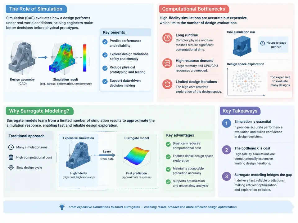
Computer-aided engineering (CAE) design optimization is the practice of driving a numerical simulation model — typically finite element analysis (FEA), computational fluid dynamics (CFD), or multibody dynamics — through a systematic search over design variables in order to improve one or more performance objectives while satisfying constraints. The simulation model is the "truth" in this loop: it encodes the physics, the geometry, and the boundary conditions, and it returns responses such as peak stress, first natural frequency, drag coefficient, or maximum temperature. The optimizer proposes candidate designs; the solver evaluates them; the loop repeats until a convergence criterion or an evaluation budget is exhausted.
This chapter establishes why that loop is expensive, where the cost actually comes from, and why surrogate modeling — also called metamodeling or response surface modeling — has become a standard engineering response. The goal is not to replace simulation but to restructure the optimization loop so that the expensive solver is called far fewer times.
The optimization loop and where simulation sits inside it
A conventional simulation-driven optimization workflow has four recurring elements. First, a parameterization step maps a vector of design variables x (for example, three sheet thicknesses and two rib heights) to a CAD or mesh update. Second, a solver run evaluates the response vector y = f(x). Third, an objective and constraint evaluation converts y into a scalar cost and a feasibility measure. Fourth, an optimization algorithm — gradient-based such as SQP, or derivative-free such as a genetic algorithm or Nelder–Mead — uses the accumulated history to propose the next x.
The critical observation is that steps two and three dominate wall-clock time, and step two dominates by orders of magnitude. A single steady-state CFD run on a 20-million-cell mesh may take 2–8 hours on 64 cores; a nonlinear explicit crash or drop simulation may take 10–30 hours. A gradient-based optimizer using finite differences needs at least n+1 solver runs per iteration for n design variables, so a 10-variable problem with 30 iterations implies roughly 330 solver calls. At 4 hours each, that is about 1,500 core-hours — and that is a modest problem.
Why the bottleneck is structural, not just a hardware problem
It is tempting to treat simulation cost as something that faster hardware will eventually solve. In practice the bottleneck is structural for three reasons. Cost scales with fidelity: design decisions often hinge on fine geometric features — fillet radii, cooling channel diameters, rib spacing — that require mesh refinement exactly where the design variables act, so higher design resolution forces higher mesh density. Cost scales with the number of variables: finite-difference gradients grow linearly with n, and adjoint methods, while far better for many-variable problems, require solver-specific implementation and are unavailable in many commercial workflows. Cost scales with non-smoothness: contact, material nonlinearity, turbulence model switching, and mesh topology changes make the response noisy or discontinuous, which degrades gradient quality and forces derivative-free methods that need even more evaluations.
There is also a workflow cost that is easy to underestimate: each solver call requires mesh regeneration, job submission, queue waiting, and post-processing. In a shared HPC cluster, queue latency alone can add hours per evaluation, so a 300-evaluation study may span weeks of calendar time even when the arithmetic says otherwise.
The surrogate modeling idea
A surrogate model is a cheap analytical approximation ŷ(x) trained on a finite set of expensive solver evaluations, called the design of experiments (DoE) or training set. Once trained, evaluating ŷ costs microseconds to milliseconds, so the optimizer can explore tens of thousands of candidates, run global search algorithms, and perform sensitivity and robustness studies that would be unaffordable with the solver in the loop.
The workflow inverts the cost structure. Instead of paying for solver calls inside every optimization iteration, you pay once for a well-chosen training set, then amortize that cost across all subsequent queries. A typical pattern is:
- Select design variables, bounds, and constraints; confirm the parameterization can regenerate a valid mesh for any x in the box.
- Generate a space-filling DoE — Latin hypercube or Sobol sequence — of, say, 60–200 points for a 5–10 variable problem.
- Run the solver at each DoE point in parallel and store x, y, and solver metadata (convergence flag, mesh quality, residuals).
- Fit a surrogate — Gaussian process (Kriging), radial basis function, polynomial response surface, or a neural network — and validate it with leave-one-out cross-validation or a held-out test set.
- Optimize on the surrogate, then verify the optimum with one or more full-fidelity solver runs.
- If verification disagrees with the surrogate prediction beyond tolerance, add the verified point to the training set and refit (adaptive sampling).
What the surrogate buys — and what it costs
The benefit is not merely speed. Because surrogate evaluation is cheap, engineers can run global optimizers that would be impractical on the solver, perform Monte Carlo robustness studies over manufacturing tolerances, generate full response surfaces for trade-off visualization, and explore multi-objective Pareto fronts. These capabilities change the nature of design reviews: instead of presenting a single optimized point, the team can present a map of feasible design space.
The cost is accuracy risk, and it must be managed explicitly. A surrogate is only valid inside the region covered by its training data; extrapolation beyond the DoE box is unreliable. Responses with sharp discontinuities — contact activation, buckling bifurcation, flow separation onset — are poorly captured by smooth global models unless the sampling is dense near the transition or the model is locally refined. The practical discipline is therefore: always validate with cross-validation before trusting the surrogate, always verify the final optimum with the full solver, and treat the surrogate as a screening and search accelerator rather than a replacement for physics.
Where this course goes
The remaining chapters build the full pipeline implied by the right-hand panel above: design variable selection and parameterization, DoE construction, surrogate model families and their inductive biases, validation metrics, adaptive sampling and infill criteria, constrained and multi-objective optimization on surrogates, and the verification loop that keeps the surrogate honest. Each technique is presented with the engineering question it answers, so that the choice of method is driven by the physics and the budget rather than by familiarity.
The central mindset to carry forward is this: simulation remains the source of truth, but the optimizer should not talk to it directly. Insert a validated, cheap approximation between them, spend the solver budget where it buys the most information, and verify the answer against the real physics before committing to a design.