1. Import and Standardize Injury Time-Histo
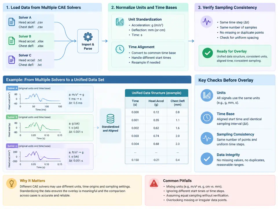
Why standardization must precede any overlay
Injury time-history work almost never starts from a single clean source. A head acceleration trace may arrive from LS-DYNA as an ASCII nodout-style export in g with a millisecond abscissa, while chest deflection comes from a RADIOSS run in mm with a microsecond abscissa, and a third curve may be a digitized sled test sampled at an irregular rate. Overlaying these directly produces curves that look plausible but are dimensionally meaningless: a 3 ms clip computed on a mis-scaled axis, or a HIC window that lands on the wrong sample count, will silently pass visual inspection and fail validation. The task in this case is therefore not plotting — it is building a single canonical representation that every downstream criterion (HIC15, 3 ms clip, deflection rate) can trust.
We define the canonical structure explicitly so later cases inherit it without renegotiation:
- Time base: seconds,
float64, strictly monotonically increasing, starting att = 0. - Acceleration: resultant magnitude in
m/s²(SI). If components are supplied, the resultant is computed after unit conversion, never before. - Deflection:
m(SI), positive convention documented per channel (chest compression positive inward). - Metadata: source solver, original units, original sampling interval, filter state (raw vs. CFC-filtered), and channel sign convention.
Loading heterogeneous sources into one record
The loader below accepts three realistic input shapes: a whitespace-delimited two-column text file, a CSV with a header, and an in-memory dict (useful when a solver API returns arrays). It normalizes units through an explicit factor table rather than guessing, and it refuses to proceed when a required unit is unknown — silent unit assumptions are the most common root cause of bad injury metrics.
import numpy as np
import csv

# Explicit, auditable conversion factors to SI
UNIT_FACTORS = {
    "time":   {"s": 1.0, "ms": 1e-3, "us": 1e-6},
    "accel":  {"m/s2": 1.0, "g": 9.80665, "mm/s2": 1e-3},
    "defl":   {"m": 1.0, "mm": 1e-3, "cm": 1e-2, "in": 0.0254},
}

def _read_two_column(path, delimiter=None):
    t, v = [], []
    with open(path, newline="") as fh:
        for row in csv.reader(fh, delimiter=delimiter):
            if not row or row[0].lstrip().startswith(("#", "//")):
                continue
            try:
                t.append(float(row[0])); v.append(float(row[1]))
            except ValueError:
                continue  # header line
    return np.asarray(t), np.asarray(v)

def load_channel(path=None, arrays=None, kind="accel",
                 time_unit="ms", value_unit="g", sign=1.0,
                 source="unknown", filtered=False):
    if arrays is not None:
        t_raw = np.asarray(arrays["t"], dtype=np.float64)
        v_raw = np.asarray(arrays["v"], dtype=np.float64)
    else:
        t_raw, v_raw = _read_two_column(path)

    if time_unit not in UNIT_FACTORS["time"]:
        raise ValueError(f"unknown time unit: {time_unit}")
    if value_unit not in UNIT_FACTORS[kind]:
        raise ValueError(f"unknown {kind} unit: {value_unit}")

    t = t_raw * UNIT_FACTORS["time"][time_unit]
    v = v_raw * UNIT_FACTORS[kind][value_unit] * sign

    order = np.argsort(t, kind="stable")
    t, v = t[order], v[order]

    return {
        "kind": kind,
        "t": t,
        "v": v,
        "meta": {
            "source": source,
            "time_unit_in": time_unit,
            "value_unit_in": value_unit,
            "sign_applied": sign,
            "filtered": filtered,
            "n_samples": int(t.size),
        },
    }
Two details matter for correctness. First, the stable sort guarantees that duplicate timestamps keep their original order, so a solver that emits repeated rows at a step boundary does not scramble the trace. Second, the sign factor is applied after unit scaling and is recorded in metadata, so a chest deflection channel exported as negative-inward can be flipped once and audited later.
Resampling onto a common time base
Overlay requires a shared abscissa, but naive interpolation hides sampling problems. The correct sequence is: (1) verify each channel is monotonic and free of duplicate times, (2) detect the native sampling interval, (3) choose a common grid at the coarsest native interval (never finer — upsampling fabricates information), and (4) interpolate with a method appropriate to the signal. For acceleration, linear interpolation is acceptable only when the native rate is well above the filter cutoff; otherwise the resampled curve will under-predict peaks. We therefore record the native interval and warn when the ratio to the target grid is unfavorable.
def native_dt(ch):
    dt = np.diff(ch["t"])
    return float(np.median(dt)), float(dt.min()), float(dt.max())

def check_sampling(ch, tol=0.02):
    dt = np.diff(ch["t"])
    if np.any(dt <= 0):
        raise ValueError(f"{ch['meta']['source']}: non-monotonic time base")
    med, lo, hi = native_dt(ch)
    jitter = (hi - lo) / med if med > 0 else np.inf
    return {"median_dt": med, "jitter_ratio": jitter,
            "uniform": jitter <= tol}

def resample(ch, t_grid):
    return {
        "kind": ch["kind"],
        "t": t_grid.copy(),
        "v": np.interp(t_grid, ch["t"], ch["v"]),
        "meta": {**ch["meta"], "resampled_from_dt": native_dt(ch)[0]},
    }

def build_common_grid(channels, t_end=None):
    dts = [native_dt(c)[0] for c in channels]
    dt_common = max(dts)                      # coarsest native rate
    t_stop = t_end if t_end is not None else min(c["t"][-1] for c in channels)
    n = int(np.floor(t_stop / dt_common)) + 1
    return np.linspace(0.0, (n - 1) * dt_common, n), dt_common
Truncating to the shortest channel end (min(c["t"][-1])) prevents extrapolation beyond a source's valid range — a frequent source of fictitious tail values in overlays. If a longer record is genuinely needed, the caller must pass t_end explicitly and accept the documented extrapolation.
Verification before overlay
Sampling consistency is verified with three independent checks, each producing a pass/fail that must be recorded alongside the data:
| Check | Condition | Failure symptom | Remedy |
|---|---|---|---|
| Monotonic time | diff(t) > 0 everywhere | Interpolation returns NaN or repeats | Stable sort; drop exact duplicates |
| Uniformity | jitter_ratio ≤ 0.02 | Peak amplitude drifts after resample | Resample to coarsest grid; flag source |
| Unit sanity | Peak accel within 0–500 g; deflection within 0–0.2 m | Values off by 1000× or 9.81× | Re-inspect value_unit and sign |
The unit sanity band is deliberately wide — it is a gross-error detector, not a physiological limit. A head acceleration peak of 3000 in the canonical structure means the source was almost certainly still in g when it should have been m/s², or vice versa.
filtered in metadata and reject re-filtering when it is already True.Reproducible walkthrough with example data
The following synthetic example exercises the full path. The numbers are illustrative, not measured: a head acceleration channel in g at 0.1 ms, a chest deflection channel in mm at 0.05 ms with an inward-negative sign, and a short digitized trace in m/s² at 0.2 ms.
t_head = np.arange(0, 0.050, 0.0001)          # 0.1 ms, 500 samples
a_head = 80.0 * np.exp(-((t_head - 0.012) / 0.004) ** 2)   # g, illustrative

t_chest = np.arange(0, 0.050, 0.00005)        # 0.05 ms
d_chest = -35.0 * np.exp(-((t_chest - 0.020) / 0.006) ** 2)  # mm, inward negative

t_sled = np.arange(0, 0.050, 0.0002)          # 0.2 ms
a_sled = 700.0 * np.exp(-((t_sled - 0.012) / 0.004) ** 2)    # m/s²

head  = load_channel(arrays={"t": t_head,  "v": a_head},
                     kind="accel", time_unit="ms", value_unit="g",
                     source="lsdyna_nodout", filtered=False)
chest = load_channel(arrays={"t": t_chest, "v": d_chest},
                     kind="defl", time_unit="ms", value_unit="mm",
                     sign=-1.0, source="radioss_csv", filtered=False)
sled  = load_channel(arrays={"t": t_sled,  "v": a_sled},
                     kind="accel", time_unit="ms", value_unit="m/s2",
                     source="sled_digitized", filtered=False)

for ch in (head, chest, sled):
    print(ch["meta"]["source"], check_sampling(ch))

grid, dt_common = build_common_grid([head, chest, sled])
head_r  = resample(head,  grid)
chest_r = resample(chest, grid)
sled_r  = resample(sled,  grid)
print("common dt [s]:", dt_common, "samples:", grid.size)
Expected observable output from this example: dt_common equals 2.0e-4 s (the coarsest native interval, from the sled trace), the grid contains 251 samples over 0–0.050 s, and each check_sampling call reports uniform: True with a jitter ratio near zero. After resampling, head_r["v"] peaks near 80 × 9.80665 ≈ 784.5 m/s² and chest_r["v"] peaks near −0.035 × (−1) = +0.035 m — the sign flip is visible and auditable in metadata. If instead the head peak prints near 80, the value_unit was left as g; if the chest peak prints near −35, the sign factor was not applied.
.npz for caching and to JSON for provenance, and every later criterion in this course consumes exactly this shape — no re-parsing, no re-guessing units.Failure symptoms and their causes
- Overlay shows one curve shifted in time. A source used a trigger offset rather than absolute time. Detect by comparing first non-zero sample; correct by subtracting the offset and recording it in metadata.
- Peak amplitude drops after resampling. The target grid was finer than native, or the native rate was too close to the signal bandwidth. Use the coarsest native interval and flag the channel.
- Deflection curve inverted. Sign convention mismatch between solvers. The
signfield makes this a one-line, auditable fix rather than an ad-hoc negation. - NaN in interpolated output. Duplicate or non-monotonic timestamps survived the sort. The stable sort handles ordering; exact duplicates must be dropped explicitly before interpolation.
With the canonical structure in place and the three checks passing, the data is ready for criterion computation. The next case consumes head_r directly to compute HIC15, which is why the time base here is in seconds and the acceleration in m/s² — the window search in that case assumes exactly these units.