1. Introduction to test scatter and model f

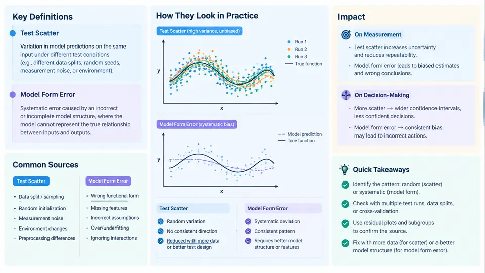
Every measurement program eventually confronts the same uncomfortable question: when a device under test (DUT) fails a specification, is the device actually bad, or is the test itself lying? Two distinct phenomena sit behind that question. Test scatter is the random, run-to-run dispersion of measured values around a stable underlying quantity. Model form error is the systematic deviation introduced when a simplified mathematical description of the measurement process — a calibration model, a behavioral model, a fixture de-embedding network, or a simulation surrogate — fails to capture the true physics of the system. Scatter is noise; form error is bias. They behave differently, they are diagnosed differently, and they corrupt decisions in different ways.

This chapter establishes the vocabulary and mental model that the remaining 29 chapters build on. The goal is not to eliminate either phenomenon — that is impossible — but to separate them so that each can be quantified, budgeted, and defended.

Definitions and the Measurement Equation

The cleanest way to formalize the distinction is through a measurement equation. Let x be the true value of the quantity of interest, and let y be the reported measurement. A general model is:

y = f(x; θ) + ε

where:
  f(x; θ)  = the measurement model (calibration curve, de-embedding
             network, behavioral surrogate), parameterized by θ
  ε        = zero-mean random error with standard deviation σ
             (test scatter)
  Δ(x)     = f(x; θ) − x  = model form error (systematic, x-dependent)

Test scatter is captured by σ and is characterized by its distribution — typically Gaussian for thermal and quantization noise, but often heavy-tailed when intermittent contacts, EMI bursts, or operator handling are involved. Model form error Δ(x) is a deterministic function of the input once θ is fixed; it does not average away with repeated measurements. This is the critical asymmetry: averaging N samples reduces scatter by √N but leaves form error untouched. A team that responds to a marginal test by simply increasing sample count will shrink the confidence interval around a biased center and may become more confidently wrong.

Where Test Scatter Comes From

Scatter sources are usually classified by whether they are internal or external to the instrument, and by their spectral character:

• Thermal noise — Johnson–Nyquist noise in the signal path; white, Gaussian, irreducible without cooling or bandwidth reduction.
• Quantization and ADC noise — deterministic in principle but effectively random relative to the signal; scales with resolution and dithering strategy.
• Source instability — reference drift, supply ripple, and phase noise that modulate the stimulus itself.
• Environmental coupling — temperature gradients, vibration, humidity, and radiated EMI entering through cables and fixtures.
• Repeatability of the interface — connector mating cycles, probe contact resistance, cable flex, and torque variation. In RF and high-speed digital work this is frequently the dominant term.
• Operator and setup variation — DUT placement, settling time allowed, and trigger configuration.

A useful discipline is to measure scatter empirically rather than assume it. A repeatability study — the same DUT, same fixture, same operator, N ≥ 30 consecutive measurements — yields a sample standard deviation that can be compared against the specification guard band. If the observed σ is comparable to a meaningful fraction of the tolerance, the test is not capable and no amount of data analysis will fix it.

Where Model Form Error Comes From

Form error arises wherever a model stands between the physical world and the reported number. Common origins:

• Linearization of nonlinear behavior — fitting a straight line to a saturating transfer function, or a first-order polynomial to a curve with significant second-order content.
• Omitted parasitic elements — ignoring fixture inductance, pad capacitance, or transmission-line loss in a de-embedding model.
• Truncated basis sets — a behavioral model (e.g., a memory-polynomial PA model) that lacks the memory depth or nonlinear order needed at the operating point.
• Interpolation and extrapolation error — calibration tables sampled too coarsely, or used outside their characterized range.
• Wrong reference plane or coordinate convention — a de-embedding that shifts the reference plane by a fraction of a wavelength produces a frequency-dependent, smoothly varying error that looks like device behavior.
• Surrogate/simulation mismatch — a compact model or ML surrogate trained on data that does not cover the corner being tested.

Form error is insidious because it is reproducible. It survives averaging, it survives re-testing on a different day, and it often survives moving to a second instrument if the same model is reused. That reproducibility is exactly what makes it dangerous: it looks like signal.

Impact on Measurement and Decision-Making

The two error types degrade decisions through different mechanisms. Scatter inflates false fails and false passes near the specification limit — a part whose true value sits at the limit will fail roughly half the time, and guard-banding is the standard remedy. Form error shifts the entire distribution, so it can produce a population that passes uniformly while every unit is wrong by the same amount, or a bimodal yield signature when the model is valid in one operating region and invalid in another.

Consider a concrete example. A power amplifier is characterized for gain at 2.4 GHz using a fixture de-embedding model built from a 2-port open/short calibration. Suppose the true gain is 18.0 dB. The fixture model omits a 0.15 dB pad loss that was not captured in the calibration standards, and the measurement scatter is σ = 0.08 dB. Over 30 repeats, the reported mean converges to 17.85 dB with a standard error of about 0.015 dB. The confidence interval is tight and entirely wrong. A yield report based on a 17.9 dB lower limit would reject a good design; a report based on 17.8 dB would pass it while masking a real 0.15 dB loss that will reappear in the customer's system. Only an independent check — a thru-line or a known artifact measured through the same path — exposes the bias.

Separating the Two: A Structural View

The figure below shows how a measured value decomposes into the true value, the model's systematic contribution, and random scatter, and how each propagates into a pass/fail decision. The key visual point is that the scatter distribution is centered on the model output, not on the true value — the offset between those two centers is the form error, and it is invisible to any statistic computed from repeated measurements alone.

What Practitioners Should Do First

Before any sophisticated analysis, establish three baselines. First, a repeatability baseline: N ≥ 30 repeats on a stable artifact, reporting mean, standard deviation, and a control chart. Second, a reference baseline: the same artifact measured through an independent path or against a traceable standard, which bounds form error. Third, a sensitivity check: perturb one suspected model input (fixture length, calibration standard, model order) and observe how much the reported value moves. If a small, physically plausible perturbation produces a shift comparable to the specification margin, form error dominates and must be addressed before scatter budgeting is meaningful.

The chapters that follow develop each of these threads: statistical characterization of scatter, model validation and residual analysis, reference-plane and de-embedding verification, guard-band design, and the decision frameworks that keep measurement uncertainty and model uncertainty from being conflated in a yield or qualification call.