1. Virtual test energy balance fundamentals
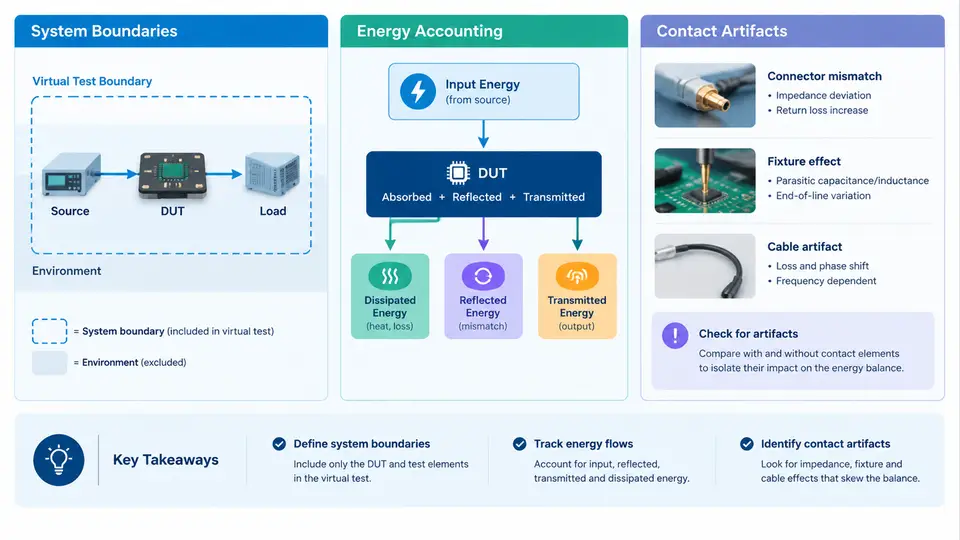
Every credible virtual test rests on a single, deceptively simple claim: the energy that enters the model must equal the energy that leaves it, plus whatever is stored or dissipated inside. When that claim fails, the simulation is not merely inaccurate — it is untrustworthy, and any conclusion drawn from it (durability margin, thermal risk, contact force peak) inherits the error. This chapter establishes the accounting framework that the rest of the course builds on: how to draw a defensible system boundary, how to book energy flows across that boundary, and how to recognize and classify the numerical artifacts that appear at contact interfaces and masquerade as physical energy sources or sinks.
Why Energy Balance Is the First Diagnostic
Displacement, velocity, and force histories are local quantities; they can look plausible while the model silently gains or loses energy. Energy balance is a global invariant, which makes it a far more sensitive detector of modeling errors. A rigid-body impact that rebounds higher than its drop height, a frictional contact that heats the system faster than the input work allows, or a penalty contact that oscillates without decaying — all of these are visible in a cumulative energy plot long before they corrupt a stress result. Treat the energy ledger as the primary acceptance gate for any virtual test, not as a post-hoc report item.
Defining the System Boundary
Energy accounting is meaningless until the control volume is fixed. In a virtual test the boundary is a modeling decision, and it must be stated explicitly before any numbers are compared. Three boundary classes cover most workflows:
- Closed boundary — no mass crosses the boundary; energy may still cross as heat or work. Typical for a sealed component under thermal-vibration loading.
- Open boundary — mass and its associated enthalpy cross the boundary, as in a cooling-circuit or exhaust-flow model. The ledger must then include flow work and advected internal energy.
- Interface boundary — the domain is split into subsystems (e.g., a suspension corner and the body it attaches to) and energy is exchanged only through defined connectors. This is the natural choice when contact artifacts are under investigation, because it isolates the interface where the artifact lives.
Whatever the class, record the boundary in the test definition: which parts are included, which are replaced by boundary conditions, and which loads are applied where. A boundary that shifts between runs invalidates any comparison of energy totals.
Sign Convention and the Energy Ledger
Adopt one sign convention and hold it for the entire test campaign. The convention used throughout this course is: energy entering the system is positive, energy leaving is negative, and stored energy is reported as a positive quantity. With that convention the balance over a time interval reads:
E_in - E_out = ΔE_stored + E_dissipated

E_in        external work (forces × displacement), prescribed heat flux, radiation in
E_out       heat loss to environment, radiation out, work done on surroundings
ΔE_stored   kinetic + internal (elastic strain, thermal) energy change
E_dissipated  friction, damping, plastic work, contact penalty losses
In practice the ledger is assembled from solver output channels: kinetic energy, internal energy, external work, contact energy, friction dissipation, and hourglass or damping energy where applicable. The residual
R(t) = E_in(t) - E_out(t) - ΔE_stored(t) - E_dissipated(t)should stay small relative to the total energy scale of the event. A practical acceptance threshold for explicit dynamic virtual tests is |R| below roughly 1–2 % of the peak total energy, with the additional requirement that R does not grow monotonically. A residual that climbs steadily indicates a numerical source; a residual that spikes at impact indicates an interface problem. Both are diagnostic, not cosmetic.
Contact Artifacts: Definition and Taxonomy
A contact artifact is any energy term, force spike, or penetration pattern at a contact interface that originates from the discretization or the contact algorithm rather than from the modeled physics. Artifacts are not automatically errors — penalty contact, for instance, is designed to store and release energy — but unaccounted artifact energy is an error. The working definition for review purposes is therefore: an interface effect whose magnitude or timing cannot be explained by the constitutive and geometric inputs of the model.
Four artifact families dominate virtual-test reviews:
| Artifact | Typical signature | Energy behavior | First check |
|---|---|---|---|
| Penetration / overclosure | Visible interpenetration at peak load | Artificial stiffness energy stored then released as a spike | Contact stiffness vs. element stiffness ratio |
| Penalty oscillation (chatter) | High-frequency force ringing at the interface | Energy pumped in and out without physical damping | Time step vs. contact frequency; damping settings |
| Hourglassing at contact | Zero-energy mesh distortion near the interface | Hourglass energy grows, often unreported | Hourglass energy channel vs. internal energy |
| Initial gap / interference | Impulse at t = 0 before any load is applied | Spurious initial kinetic energy injection | Geometry clearance audit and initial penetration report |
The taxonomy matters because each family is diagnosed differently. Penetration is a stiffness-scaling question; chatter is a time-integration question; hourglassing is a mesh-quality question; initial interference is a geometry-hygiene question. Classifying the artifact before adjusting any parameter prevents the common failure mode of tuning contact stiffness to hide a meshing defect.
Worked Example: Impact of a Bracket onto a Rigid Plate
Consider a steel bracket of 0.8 kg released from 0.25 m onto a rigid plate, modeled with a penalty contact and an explicit solver. The initial kinetic energy at first contact is mgh ≈ 0.8 × 9.81 × 0.25 ≈ 1.96 J. The test definition fixes the boundary as the bracket alone, with the plate represented as a rigid boundary condition, and adopts the sign convention above.
Run the model and extract the energy channels at 1 ms intervals. Expected observations for a sound model: kinetic energy falls to near zero at peak compression, internal (strain) energy peaks at roughly the impact energy minus friction losses, contact energy returns to near zero after separation, and the residual stays under 2 % of 1.96 J. If instead the contact energy channel retains 0.3 J after separation, the interface is storing energy that never returns — a penalty artifact. If hourglass energy exceeds about 5 % of internal energy, the mesh under the contact patch is too coarse or poorly shaped. If a force spike appears in the first increment, audit the initial gap: a 0.05 mm interference on a stiff penalty contact can inject an impulse comparable to a measurable fraction of the impact energy.
Practical Review Sequence
- State the boundary class and the sign convention in the test record.
- Plot all energy channels on one normalized axis; confirm the residual stays within threshold and does not trend upward.
- Inspect the contact energy channel specifically for energy retained after separation.
- Compare hourglass and damping energy against internal energy; flag ratios above the project threshold.
- Audit initial penetration and gap reports before interpreting any force peak.
- Classify any anomaly using the artifact taxonomy, then correct the root cause rather than the symptom.
The figure above ties the three concepts together: the boundary fixes what is counted, the ledger fixes how it is counted, and the artifact taxonomy fixes what to do when the ledger does not close. In the next chapters these fundamentals are applied to specific test types, but the invariant remains the same — if the energy does not balance, the virtual test has not yet earned the right to be believed.