1. Load cell fundamentals

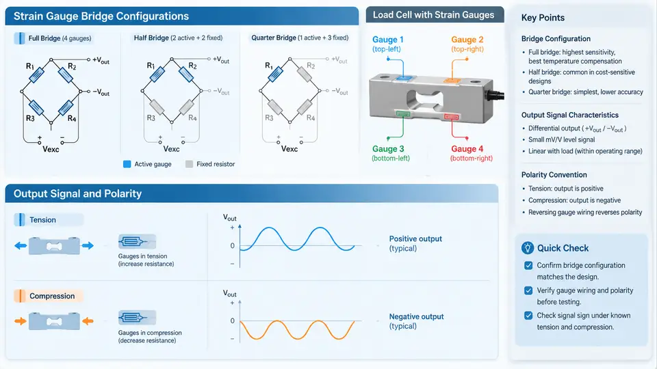
A load cell converts a mechanical force into a measurable electrical signal. Almost every industrial load cell used in weighing, force feedback, and tension control relies on the same core principle: a metal or alloy element deforms elastically under load, and bonded strain gauges convert that deformation into a change in electrical resistance. Understanding the bridge configuration, the nature of the output signal, and the sign conventions used for tension and compression is the foundation for every later task in this course — verifying polarity and confirming that each channel is mapped to the correct physical axis.

Strain gauges and the Wheatstone bridge

A metallic strain gauge is a thin foil pattern bonded to a substrate. When the substrate stretches, the foil lengthens and narrows, and its resistance increases; when it compresses, the resistance decreases. The fractional resistance change is small — typically on the order of 0.1 % at full rated load — so a single gauge is impractical to read directly. Instead, gauges are wired into a Wheatstone bridge, where four arms are excited by a stable DC voltage (commonly 5 V or 10 V) and the differential voltage across the bridge midpoints is measured.

The bridge output is approximately proportional to the excitation voltage and to the algebraic sum of the strain in the four arms:

V_out ≈ V_exc · (GF / 4) · (ε1 − ε2 + ε3 − ε4)

where GF is the gauge factor (about 2.0 for constantan foil) and ε is strain. The signs in that expression are the key to everything that follows: gauges that are stretched contribute positively, gauges that are compressed contribute negatively, and the wiring order determines which arm is which. A well-designed load cell places gauges so that the wanted load produces a large differential output while unwanted effects — temperature, axial off-axis force, and bending in the wrong plane — cancel or largely cancel.

Common bridge configurations

Three configurations appear in practice, and each has a distinct output characteristic:

• Quarter bridge — one active gauge and three fixed resistors. Output is roughly one quarter of the full-bridge sensitivity, and temperature compensation is poor. Rare in commercial load cells, common in laboratory demonstrations.
• Half bridge — two active gauges, usually one in tension and one in compression, placed in adjacent arms. Temperature effects on the two gauges tend to cancel, and sensitivity is doubled relative to a quarter bridge.
• Full bridge — four active gauges, two stretched and two compressed under the intended load. This is the standard for beam, column, S-type, and pancake load cells. Sensitivity is four times the quarter-bridge value, temperature compensation is excellent, and the bridge is naturally insensitive to axial thermal expansion.

In a typical bending-beam cell, gauges 1 and 3 sit on the top surface and gauges 2 and 4 on the bottom. Under a downward load the top surface stretches and the bottom compresses, so the bridge produces a clean differential output. If the same cell is loaded upward, every gauge reverses its strain and the output reverses sign — a fact that becomes central when polarity is verified.

Output signal characteristics

Load cell datasheets express sensitivity in millivolts per volt of excitation at rated capacity, for example 2.0 mV/V. With 10 V excitation, a 2.0 mV/V cell therefore produces 20 mV at full rated load. That is a small signal, and it is why load cell inputs on weighing terminals and DAQ modules are designed as low-level differential inputs with high common-mode rejection, often with a ratiometric measurement that uses the excitation voltage as the ADC reference so that supply drift cancels.

Several characteristics matter when you later verify polarity and channel mapping:

• Zero offset — the output at no load, specified as a percentage of rated output (e.g. ±1 % RO). It is not a fault; it is trimmed in software or by the terminal's zero command.
• Creep and drift — slow output change under constant load or temperature; relevant when a reading seems to wander during a long verification.
• Non-linearity and hysteresis — deviation from a straight-line response and difference between loading and unloading curves, usually below 0.05 % RO for good cells.
• Input and output resistance — typically 350 Ω or 1000 Ω bridges; useful for identifying the excitation pair versus the signal pair when wiring is undocumented.

Polarity conventions for tension and compression

Polarity is a convention, not a physical absolute, and it must be defined before it can be verified. The convention used throughout this course is:

• Positive output corresponds to tension (the cell is pulled, or the load acts in the direction that stretches the primary gauges).
• Negative output corresponds to compression (the cell is pushed, or the load compresses the primary gauges).
• The signal is measured as V_SIG+ − V_SIG−, with the excitation applied as V_EXC+ to V_EXC−.

This matches the common industrial convention in which a tension load produces a positive reading on a weighing terminal. However, manufacturers differ: some S-type cells are wired so that a downward pull gives positive output, others the reverse, and the wire colour code (red/black for excitation, green/white for signal is common but not universal) varies between vendors. The only reliable rule is to consult the datasheet and then confirm by test.

A practical verification uses a known load and a known direction. With the cell mounted and the terminal zeroed, apply a small known mass or use a calibrated force gauge in the tension direction. The displayed value should increase positively and scale roughly linearly with the applied load. Reverse the direction to compression; the reading should go negative by a similar magnitude. If the sign is inverted, the fix is either to swap the two signal wires at the terminal or to invert the channel in software — but only one of these, and it must be recorded so that later channel-mapping checks are not confused by an undocumented inversion.

From bridge to channel: what the signal chain looks like

The figure below traces the signal from the bridge through the conditioning and conversion stages to the mapped channel, and shows where polarity is established and where it can be lost.

Two points in that chain deserve emphasis. First, the polarity is physically established at the bridge and preserved by the differential amplifier; everything downstream is a faithful copy unless someone deliberately inverts it. Second, the channel map is a separate layer: a correctly polarized signal can still appear on the wrong axis if the wiring to the terminal or the software mapping is crossed. That is why this course treats polarity verification and channel mapping verification as two distinct but linked checks — the first confirms sign, the second confirms identity.

A worked orientation example

Consider a three-axis platform with three beam-type load cells, each rated 500 N and 2.0 mV/V, connected to a terminal with 10 V excitation and a gain that yields 20 000 counts at full load. With the platform unloaded, the terminal is zeroed. A 100 N calibration mass is then placed at the centre of the platform, and the expected reading on each axis is approximately:

Expected counts = (100 N / 500 N) × 20 000 = 4 000 counts

If the Z-axis channel reads +4 000 counts, the sign and scale are consistent with the tension-positive convention for that axis. If it reads −4 000 counts, the signal pair is reversed relative to the convention — correct it at the signal wires or in software, and record the change. If the X-axis channel responds instead of Z, the channel map is crossed and must be corrected before any further testing. If the reading is near zero on all channels, suspect the excitation or a broken gauge lead rather than a polarity problem.

These three outcomes — correct sign, inverted sign, and wrong channel — are exactly the failure modes that the rest of this course is built to detect systematically. With the bridge behaviour, the millivolt-level output, and the tension-positive convention clearly in mind, the next step is to turn those principles into a repeatable verification procedure.