1. High-speed video synchronization landsca

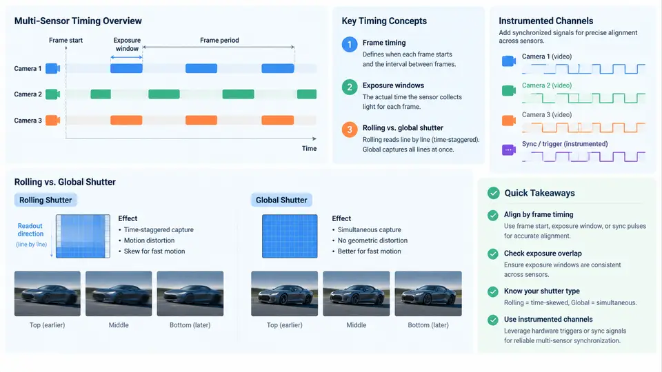
High-speed video synchronization is the discipline of ensuring that every frame captured by every camera in a system can be placed on a common, trustworthy timeline. In a single-camera setup this is mostly a matter of knowing when each frame started and how long the sensor was exposed. In a multi-sensor system — stereo rigs, surround-view arrays, machine-vision cells with four to sixteen cameras, or a high-speed camera paired with a LiDAR and an inertial measurement unit — the problem becomes one of cross-device causality: which pixel in camera A corresponds to which pixel in camera B, and to which sample of the IMU, within a tolerance the downstream algorithm can tolerate.

The word "high-speed" changes the stakes. At 1,000 fps a frame period is 1 ms; at 10,000 fps it is 100 µs. A synchronization error that would be invisible at 30 fps — say 200 µs — is two full frames at 10 kHz. Motion blur, rolling-shutter skew, and trigger latency all scale into the same order of magnitude as the frame period, so the synchronization budget must be designed rather than assumed.

Frame timing and the exposure window

Every frame has three distinct time markers that are often conflated: the trigger instant (when the camera is told to start a frame), the exposure window (the interval during which photons are integrated), and the readout window (when charge is digitized and transferred). For a global-shutter sensor the exposure window applies to all pixels simultaneously, so a single timestamp — usually the midpoint of the exposure — is a faithful description of the frame. For a rolling-shutter sensor each row has its own exposure window, offset by a row time that is typically a few microseconds to tens of microseconds. The frame's "timestamp" is then only a convention, and the convention must be stated explicitly: first-row start, mid-frame, or last-row end.

A useful mental model is a timing budget. If the application requires that two cameras observe the same physical event within Δt, then the sum of trigger skew, exposure-window mismatch, and timestamp quantization must stay below Δt. For a 500 fps stereo pair with a 50 µs tolerance, a 10 µs trigger skew and a 20 µs timestamp quantization already consume 60% of the budget before any optical or algorithmic error is considered.

Rolling versus global shutter in synchronized systems

Global shutter is the natural choice for synchronization because a frame is a well-defined instant. Rolling shutter is cheaper and often faster in terms of frame rate, but it introduces a spatial-temporal gradient: the top of the image is captured earlier than the bottom. In a multi-camera system this gradient interacts with geometry. Two rolling-shutter cameras that are perfectly trigger-aligned still disagree about the scene if their readout directions differ, and a rolling-shutter camera synchronized to a global-shutter camera has a time-varying offset across the image.

The practical consequence is that rolling-shutter cameras can be synchronized, but the synchronization must be row-aware. The line time (the time between consecutive row starts) is a datasheet parameter, and the per-row timestamp is t_row = t_first_row + row_index × t_line. Any fusion or triangulation step that assumes a single timestamp per frame will introduce a bias proportional to the line time and the row index. For high-speed work, this bias is frequently larger than the trigger jitter the team is trying to eliminate.

Why instrumented channels matter

An instrumented channel is a hardware path that carries timing information alongside the video data — a dedicated trigger line, a GPIO strobe, a PTP-disciplined Ethernet timestamp, or an embedded timecode in the transport stream. Its purpose is to make the synchronization observable and verifiable rather than inferred. Without an instrumented channel, a team can only assume that the trigger arrived; with one, the arrival can be measured, logged, and compared across devices.

Instrumented channels serve three roles. First, they distribute a common time base: a PTP grandmaster, a GPS-disciplined oscillator, or a shared hardware trigger. Second, they carry event markers: a strobe LED in view, a GPIO pulse recorded by a data logger, or a timestamp embedded in each frame's metadata. Third, they provide a verification path: an oscilloscope or logic analyzer can capture the trigger edges at each camera and reveal skew, jitter, and dropped triggers that no amount of software timestamping would expose.

Putting the pieces together

The diagram below shows the timing relationships that a synchronization design must control. A master time base feeds a trigger distributor; each camera exposes its frame within a window whose position and width are set by the trigger and the exposure configuration; the instrumented channel records the actual edge at each device so that the assumed and actual timing can be compared.

Read the timing view from left to right. All three cameras receive the trigger edge at the same nominal instant, but the global-shutter cameras expose a single 200 µs window while the rolling-shutter camera exposes successive rows across a much longer span. If the application fuses the three images as if they were simultaneous, the rolling camera's lower rows will be temporally displaced by up to the full readout duration. The instrumented channel is what lets the team see this displacement as a measured quantity rather than a theoretical worry.

Design implications for multi-sensor systems

Three practical rules follow from the landscape above. First, define the timestamp convention before writing any fusion code: state whether a frame's time is the trigger edge, the exposure midpoint, or the first-row start, and apply that convention consistently across every device and every log. Second, budget the skew explicitly: allocate the total tolerance among trigger distribution, exposure mismatch, timestamp quantization, and transport latency, and verify each allocation with the instrumented channel. Third, treat rolling-shutter cameras as row-timestamped devices, not as frame-timestamped ones; if the fusion algorithm cannot consume per-row timestamps, either restrict the rolling camera to low-motion scenes or replace it with a global-shutter device.

A concrete verification step makes these rules tangible. Configure the trigger distributor to emit a 1 kHz pulse, connect the pulse to a visible LED in the scene and to a logic analyzer channel, and record the LED edge in each camera's field of view. The frame in which the LED transition appears gives the camera's effective latency; the difference between cameras gives the residual skew. If the measured skew exceeds the budget, the logic analyzer trace will show whether the error originates in the distributor, in a cable, or in a camera's internal trigger delay — a diagnosis that host-side timestamps alone cannot provide.

With the landscape established — frame timing, exposure windows, shutter behavior, and the measurement role of instrumented channels — the remaining chapters can build on a shared vocabulary. The next design decisions concern how the time base is generated and distributed, how triggers are physically routed, and how the resulting timing is validated against the application's tolerance.