1. Virtual buck and sled evidence in early
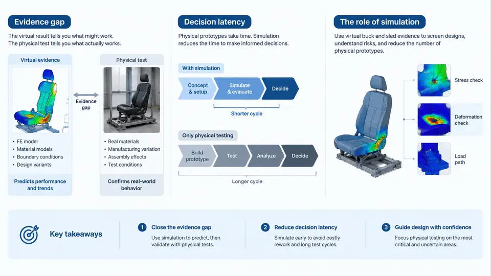
Early hardware programs rarely fail because engineers cannot build a buck. They fail because the program commits to a mechanical architecture, a power topology, or a thermal envelope before anyone has produced credible evidence that the design will survive its own operating conditions. The first chapter of this course establishes the vocabulary and the decision framework that the remaining chapters build on: what counts as evidence in early design, where the evidence gap comes from, how decision latency accumulates, and why a virtual buck and sled — a simulation-backed representation of the converter and its load/test fixture — is the cheapest instrument for closing that gap before the first physical prototype exists.
What "Buck" and "Sled" Mean as Evidence Objects
In this course, buck refers to the switching step-down converter under design — its power stage, control loop, sensing, and protection behavior. Sled refers to the electrical and thermal load fixture that the buck drives during validation: the programmable electronic load, the harness, the current-sense shunts, the bulk and decoupling network, and the thermal mass that determines how fast the load can be stepped. A sled is not a passive accessory; its impedance, inductance, and thermal time constants materially change what the buck "sees" and therefore what the measured waveform means.
Evidence, then, is any observation that reduces uncertainty about a design decision. A simulation result is evidence only when it is traceable to a model, a stimulus, and an acceptance criterion. A number without a criterion is data, not evidence. This distinction matters because early programs are flooded with data (duty cycle plots, efficiency curves, transient screenshots) and starved of decisions that can be defended.
The Evidence Gap in Early Design
The evidence gap is the distance between the confidence a decision requires and the confidence the available artifacts actually provide. In a typical program, the gap is widest exactly when the most expensive commitments are made. Mechanical tooling, connector selection, PCB layer count, and thermal interface choices are locked in months before a prototype can be measured. At that moment the team has:
- datasheet typicals and vendor reference designs, which describe someone else's board, not yours;
- spreadsheet calculations that assume ideal components and a fixed ambient;
- bench data from a previous, differently loaded platform;
- and no measurement of the actual buck–sled interaction.
The gap is not a knowledge problem; it is a timing problem. The information needed to decide arrives after the decision is due. Simulation exists to move that information earlier, not to replace measurement.
Decision Latency and Why It Compounds
Decision latency is the elapsed time between the moment a decision becomes necessary and the moment it can be made with adequate evidence. It is not the same as engineering effort. A team can work intensely for six weeks and still have high latency if the evidence they need depends on a build that has not been scheduled.
Latency compounds because design decisions are coupled. A late decision on the buck's switching frequency delays the inductor selection, which delays the thermal stack-up, which delays the enclosure, which delays the sled harness routing. Each downstream decision inherits the upstream delay and adds its own. The result is a program that appears to be "in design" for a long time and then compresses all real decisions into a short, high-risk window just before tooling release.
Virtual evidence attacks latency directly. A parameterized simulation of the buck and sled can answer "what happens if we drop from 500 kHz to 350 kHz?" in hours rather than in a build cycle. The value is not the accuracy of the model in absolute terms; it is the relative ranking of options under identical, controlled stimuli. That ranking is usually enough to commit to an architecture and defer fine-tuning to hardware.
Where Simulation Earns Its Place — and Where It Does Not
Simulation is not a substitute for measurement, and treating it as one is the most common way virtual evidence loses credibility. The defensible role of simulation before prototypes is narrower and more useful:
| Question type | Simulation role | Physical prototype role |
|---|---|---|
| Architecture selection (topology, frequency, phase count) | Primary — compare options under identical stimuli | Confirmation only |
| Control-loop stability margin | Primary — sweep gain/phase across load and line | Verify on the real plant |
| Transient response to a defined load step | Strong — with a sled model that includes harness L and load slew rate | Authoritative |
| Thermal steady state and hot-spot location | Directional — geometry and boundary conditions dominate | Authoritative |
| EMI signature | Weak — layout parasitics and near-field coupling are not captured | Authoritative |
| Component tolerance and worst-case yield | Strong — Monte Carlo over parameter distributions | Sampled verification |
The pattern is consistent: simulation is strongest where the physics is well-bounded and the stimulus can be defined precisely, and weakest where parasitic geometry and field coupling dominate. A credible early-design plan assigns each decision to the instrument that can actually close it, rather than defaulting everything to "we'll see on the bench."
A Worked Example: Closing a Transient-Response Gap
Consider a 48 V to 12 V, 20 A buck feeding a sled whose load can slew at 5 A/µs. The program must decide whether a single-phase design with 470 µF of output capacitance meets a ±150 mV transient window, or whether a two-phase design is required. The physical prototype is eight weeks out.
The virtual buck is built with the actual controller model, the selected inductor's saturation curve, and a sled model that includes 1.2 µH of harness inductance and the load's finite slew rate. The stimulus is a 5 A to 15 A step at 5 A/µs, repeated at three input voltages (42 V, 48 V, 54 V) and two ambient temperatures. The acceptance criterion is the same one the bench will use: peak deviation ≤ 150 mV and recovery within 200 µs.
# Example simulation sweep definition (illustrative parameters)
stimulus:   load_step 5A -> 15A, slew 5 A/us
conditions: Vin = {42, 48, 54} V, Ta = {25, 85} C
metrics:    Vpeak_dev, t_recover, phase_margin
criterion:  Vpeak_dev <= 150 mV AND t_recover <= 200 us
sweep:      phases = {1, 2}, Cout = {470u, 660u} F
The sweep shows the single-phase case exceeding the window at 42 V and 85 °C, while the two-phase case with 470 µF meets it with margin. The decision is made in days, the tooling proceeds on a two-phase layout, and the bench later confirms the ranking — even if the absolute peak deviation differs by 10–15%, which is expected and acceptable. The point is that the decision was correct, not that the model was exact.
The Evidence Gap, Latency, and Simulation as One System
The three concepts are inseparable. The evidence gap defines what is missing; decision latency defines when it is needed; simulation defines how it can be produced early enough to matter. The diagram below shows how a decision's required confidence, the available evidence, and the time-to-evidence interact, and where virtual buck and sled evidence inserts into that chain.
The diagram makes the central argument of this chapter visible: the required-confidence curve rises steeply as architecture freezes, while physical-build evidence arrives late and slowly. The shaded region between them is the evidence gap, and the horizontal bracket is the decision latency it creates. Virtual buck and sled evidence does not eliminate the gap — it inserts a controlled, traceable source of evidence into the early window, compressing latency and letting the program commit to an architecture with a defensible rationale rather than a hopeful one.
What This Chapter Establishes for the Rest of the Course
Three commitments follow from the framework above and recur throughout the course. First, every simulation must be tied to a named decision, a defined stimulus, and an explicit acceptance criterion; otherwise it is decoration. Second, the sled must be modeled as part of the system, not as an ideal load, because the buck–sled interaction is where most early surprises originate. Third, virtual evidence is used to rank and commit, not to certify; certification remains the job of the physical prototype, and the course treats the handoff between the two as a designed transition rather than an abrupt switch.
With the evidence gap, decision latency, and the role of simulation defined, the next step is to make the virtual buck and sled concrete: what models are needed, what fidelity each decision requires, and how to build a simulation setup that produces evidence a program can actually act on.