1. PAM-CRASH in HPC environments
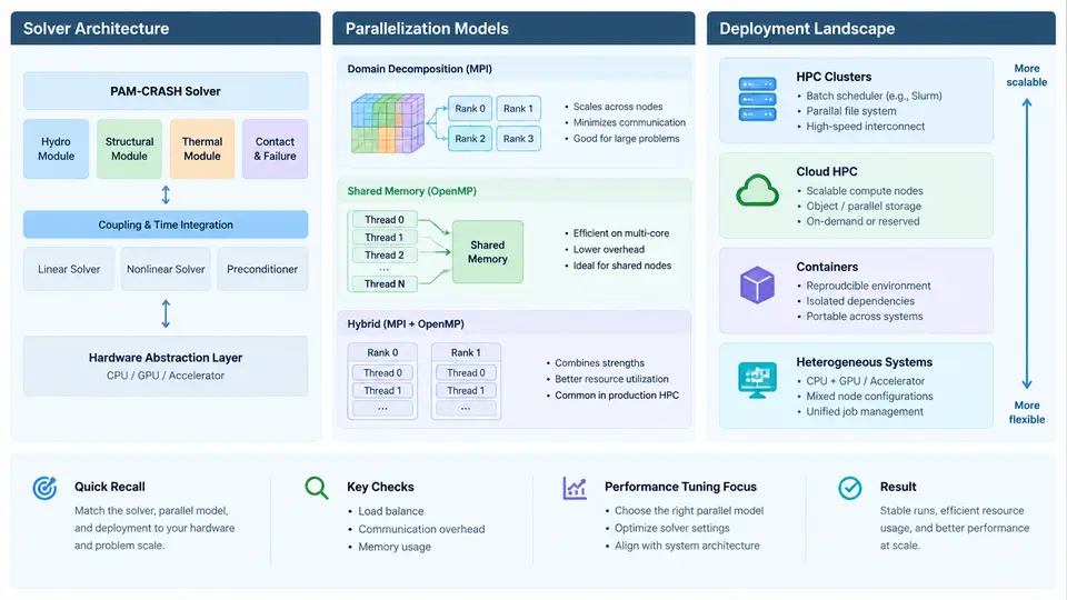
PAM-CRASH is an explicit finite element solver used primarily for crashworthiness, occupant safety, and impact simulation in the automotive and aerospace industries. Its computational profile is dominated by short time steps, contact-intensive workloads, and highly nonlinear material behavior. Understanding how the solver is structured internally, how it distributes work across processors, and where it typically runs in production is a prerequisite for any meaningful performance tuning effort. This chapter establishes that foundation.
Solver Architecture
PAM-CRASH follows the classical explicit dynamics architecture. The central loop advances the solution in time using the central difference method, where the stable time step is governed by the Courant–Friedrichs–Lewy condition applied to the smallest element in the mesh:
dt_critical = 2 / omega_max
omega_max  ~ sqrt(k / m)   (highest element eigenfrequency)
Because the time step is bounded by the smallest element, mesh quality directly controls total runtime. A single degenerate element can reduce the global time step by an order of magnitude, which is why mesh conditioning is treated as a performance concern rather than a purely modeling concern.
Each time step executes a fixed sequence of phases: element force computation, hourglass control, contact detection and force assembly, nodal force summation, and state update. The element force computation is embarrassingly parallel because each element only reads its own nodes and material state. Contact, by contrast, is the dominant scalability bottleneck. Contact search must identify candidate node-to-segment or segment-to-segment pairs, and the cost grows with the number of active contact interfaces and the surface area involved.
PAM-CRASH supports multiple element formulations (shells, solids, beams, spot welds, airbags) and material models (metals with strain-rate dependence, foams, composites, fabrics). Each formulation carries its own computational cost per element, so the element type mix in a model strongly influences which hardware configuration is optimal.
Parallelization Models
PAM-CRASH offers two primary parallelization strategies, and choosing between them is one of the most consequential deployment decisions.
Shared-memory (SMP) parallelization uses OpenMP threads within a single compute node. The domain decomposition is implicit: all threads access the same global mesh, and parallelism is expressed at the loop level over elements and nodes. SMP scales well up to the core count of a single socket or node, typically 32–64 cores on modern hardware, but does not extend across nodes. Its advantage is simplicity: no domain decomposition overhead, no MPI communication, and no partitioning artifacts in contact results.
Distributed-memory (MPP) parallelization uses MPI ranks with explicit domain decomposition. The mesh is partitioned into subdomains, each assigned to a rank. Nodes on subdomain boundaries are duplicated as ghost nodes, and forces are exchanged each time step. MPP scales to hundreds or thousands of cores, but introduces communication overhead that grows with the surface-to-volume ratio of subdomains. Contact interfaces that cross subdomain boundaries are particularly expensive because contact pairs must be communicated.
Hybrid MPI+OpenMP configurations are also supported, where each MPI rank spawns multiple OpenMP threads. This is often the best choice on clusters with many-core nodes, as it reduces the number of MPI ranks (and thus communication volume) while still exploiting intra-node parallelism.
Deployment Landscape
PAM-CRASH is deployed across three broad environments: on-premise clusters, cloud HPC instances, and workstation-class local runs. Each has distinct characteristics.
On-premise clusters typically use InfiniBand interconnect (EDR, HDR, or NDR) with MPI implementations such as Intel MPI, OpenMPI, or Platform MPI. Job submission goes through schedulers like SLURM, PBS Pro, or LSF. The critical deployment parameters are the MPI fabric configuration, the placement of ranks relative to NUMA domains, and the shared filesystem used for scratch I/O.
Cloud HPC instances offer elastic capacity but introduce variability in interconnect performance and storage latency. Instance families with high-bandwidth networking (for example, those with EFA or RoCE) are preferred for MPP runs. The main tuning concern is ensuring that the instance's network bandwidth does not become the bottleneck for ghost-node exchange.
Workstation-class runs are common for model debugging and small sub-assembly simulations. These are almost always SMP, and the primary concern is memory bandwidth rather than interconnect.
The following diagram summarizes the relationship between solver phases, parallelization strategy, and the deployment environments where each is typically used.
Practical Implications for Deployment
The architecture and parallelization model directly determine what to check before a production run. Three items deserve attention on every new deployment.
Memory per rank. MPP runs duplicate ghost nodes and contact data on each rank. A model that fits in 8 GB on a single node may require 12–16 GB per rank after decomposition. Underestimating this leads to out-of-memory kills that are often misdiagnosed as solver crashes.
Partition quality. The domain decomposition tool should produce subdomains with roughly equal element counts and minimal boundary surface. A poor partition creates load imbalance and excessive ghost-node communication. Checking the partition report for element count variance and boundary node count is a quick sanity check.
Contact interface placement. If a critical contact interface (for example, a barrier-to-vehicle interface) is split across many subdomains, communication cost spikes. Some deployments deliberately align subdomain boundaries with non-contact regions to avoid this.
What to Carry Forward
The explicit time-step loop, the SMP versus MPP trade-off, and the three deployment environments form the conceptual map for everything that follows in this course. Performance tuning is not a generic activity; it is the practice of identifying which phase of the loop is limiting, which parallelization strategy is in use, and which deployment constraint is binding. The next chapters will build on this map to address specific tuning techniques for each phase and each environment.