1. Course overview

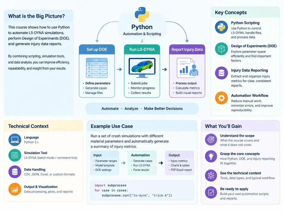
This course addresses a recurring bottleneck in crashworthiness and structural-impact engineering: the manual effort required to turn a large family of LS-DYNA simulations into a defensible design-of-experiments (DOE) study and a set of injury-metric reports. A typical occupant-protection or barrier-impact program may require dozens to hundreds of runs, each varying restraint parameters, material properties, or impact conditions, and each producing binary plot files, ASCII result databases, and time-history curves. Doing this by hand is slow, error-prone, and difficult to audit. The goal here is to replace that manual loop with a reproducible Python toolchain that generates input decks, dispatches solver runs, extracts response quantities, and assembles the statistical and regulatory outputs.

The scope is deliberately end-to-end but bounded. We cover the automation layer around LS-DYNA, not LS-DYNA solver theory itself. You are expected to be comfortable with explicit dynamic analysis concepts — hourglass control, contact definitions, time-step scaling — but the course focuses on how to drive the solver programmatically, how to parse its outputs reliably, and how to structure the resulting data so that statistical analysis and reporting are trustworthy. Finite element model debugging, mesh quality, and material calibration are treated as inputs to the workflow, not as topics of instruction.

The three technical pillars

The course is organized around three interlocking capabilities, and understanding how they connect is the single most important conceptual step in this chapter.

• DOE orchestration. A sampling plan (full factorial, Latin hypercube, or optimal design) defines the parameter combinations to run. Python generates one keyword deck per run by templating a baseline model, substituting parameter values into specific *PARAMETER cards or include files, and writing each deck to its own run directory.
• Solver execution and monitoring. Runs are launched via subprocess or a job scheduler, with exit-status checks, d3hsp and messag file scanning for termination and warning conditions, and restart handling for failed runs.
• Response extraction and reporting. Time-history data (accelerations, forces, displacements) and derived injury criteria are read from binout or ASCII output, reduced to scalar responses per run, and then fed into regression, sensitivity analysis, and formatted report generation.

These pillars share a common data contract: every run must be identifiable by its parameter vector, and every extracted response must be traceable back to that run. If that contract breaks — for example, if a run directory is overwritten or a response is matched to the wrong deck — the entire statistical conclusion becomes invalid, often silently. Much of the engineering discipline in this course exists to protect that traceability.

Injury criteria in context

Because the reporting target is injury data, the course uses established occupant-safety metrics as its worked responses. The Head Injury Criterion (HIC) is computed from the resultant head acceleration time history over a 36 ms window:

HIC = max over t1,t2 of [ (t2 - t1) * ( (1/(t2-t1)) * ∫ a(t) dt )^2.5 ]
      with t2 - t1 ≤ 36 ms, a(t) in g

Other responses used in examples include the 3 ms chest acceleration clip, chest deflection, and the Neck Injury Criterion (Nij). The exact formulas matter less at this stage than the data-handling implication: each criterion is a nonlinear functional of a sampled time history, so the extraction code must handle sampling intervals, filtering (typically SAE J211 Class 180 or Class 600), and window search correctly. A HIC value computed from unfiltered or wrongly resampled data can differ by tens of percent from the regulated value, which is why the extraction layer is treated as a validated component rather than a convenience script.

How the pieces fit together

The diagram below shows the full data path from baseline model to final report, including the two feedback points where automation most often needs engineering judgment: the run-health gate after solver execution, and the response-validation gate before statistical analysis.

What "reproducible" means in practice

A DOE study is only as good as its ability to be re-run and audited. Three concrete practices are established from the first chapter and used throughout. First, every run directory contains a copy of the exact deck that was executed, not a reference to a template — templates change, and a study must remain reconstructable. Second, the run matrix is a versioned CSV whose rows carry a stable run_id, and every extracted response table joins back to that ID. Third, solver version, Python environment, and extraction-script version are recorded in a manifest alongside the results. When a reviewer asks why run 47 produced an anomalous HIC, the answer should be recoverable from the directory tree alone.

Prerequisites and tooling

The examples assume Python 3.10 or later with numpy, pandas, scipy, matplotlib, and lasso-python (the LS-DYNA Python reader for binout and d3plot data). Deck templating uses plain string handling or jinja2; job dispatch uses subprocess locally and is shown in a scheduler-agnostic form so it can be adapted to Slurm or PBS. On the LS-DYNA side, you need a working solver installation and a baseline model that runs to normal termination before any automation begins — automating a model that does not converge simply produces many failed runs faster.

By the end of the course you will have built a small, complete pipeline: a parameterized baseline deck, a sampling plan of roughly 20–40 runs, an extraction module validated against a reference case, a sensitivity analysis, and a formatted injury-response report. The scale is intentionally modest so that every stage can be inspected and understood; the same structure scales to hundreds of runs without architectural change.