1. Introduction to tolerance studies in occ

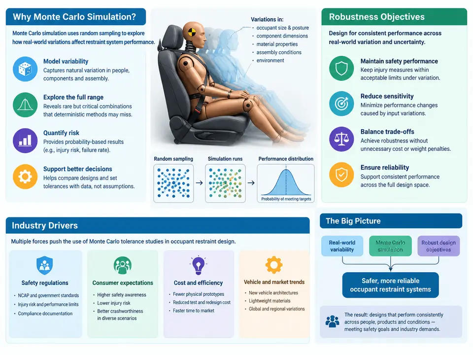
Occupant restraint design has always been a nominal-value discipline in its first approximation: an engineer selects an airbag inflator output, a seat belt load limiter level, a pretensioner stroke, and a knee bolster stiffness, then verifies the resulting occupant response against regulatory and consumer-metric targets. That nominal design is necessary but never sufficient. Every physical input to a crash model carries manufacturing spread, material batch variation, sensor and instrumentation uncertainty, and modeling error. A restraint system that passes FMVSS 208 or Euro NCAP at nominal values can still fail in a meaningful fraction of the real vehicle population if those variations push the occupant response across a compliance threshold. Tolerance studies exist to quantify that fraction before hardware exists, and Monte Carlo simulation is the workhorse method for doing so.

Why nominal-only validation is structurally insufficient

Consider a driver-side frontal 56 km/h rigid barrier event. The occupant injury metrics of interest — HIC15, chest deflection, neck Nij, and femur load — are nonlinear, threshold-governed responses. Small changes in belt payout, D-ring geometry, or inflator burn rate do not produce proportional changes in chest deflection; they interact with the occupant's forward excursion, the airbag's unfolding trajectory, and the timing of belt spool-out. The result is that the response surface is curved and often has local steep regions. A design point sitting comfortably inside the corridor at nominal values may be only a few percent away from a limit in a direction that manufacturing variation explores routinely.

Deterministic worst-case studies — running a handful of hand-picked "worst" combinations — are also unreliable. With ten or more uncertain inputs, the true worst case is rarely the combination of each input's individual extreme, because the response is not monotonic in every variable. Monte Carlo sampling explores the joint distribution and reveals the actual tail behavior rather than an assumed one.

What Monte Carlo simulation contributes

A Monte Carlo tolerance study replaces each uncertain input with a probability distribution, draws N samples from the joint input space, runs the crash or occupant simulation for each sample, and treats the resulting set of responses as an empirical distribution. From that distribution the engineer extracts the quantities that matter for a robustness decision:

• Probability of non-compliance — the fraction of samples exceeding a regulatory or target threshold, e.g. chest deflection above 42 mm.
• Statistical margins — the distance from the nominal response to the limit expressed in standard deviations or in percentiles (P95, P99), not in absolute millimeters alone.
• Input sensitivity ranking — correlation or variance-based measures that identify which tolerances dominate the output spread, directing tolerance tightening or design changes where they pay off.
• Tail shape — whether the response distribution is symmetric, skewed, or heavy-tailed, which determines whether a mean-plus-two-sigma rule of thumb is defensible.

The practical value is not a single number but a decision: whether to release the design, tighten a supplier tolerance, add a design margin, or change the restraint architecture. A study that reports "P99 chest deflection = 38.4 mm against a 42 mm limit" supports a release decision in a way that a nominal run of 34 mm cannot.

Robustness objectives and how they are stated

A robustness objective is a statement about the response distribution, not about a single run. In restraint engineering the objective is usually expressed in one of three forms. The first is a probability target: "probability of exceeding 42 mm chest deflection must be below 1% across the production population." The second is a statistical margin: "the P99 response must sit at least 10% below the regulatory limit." The third is a sensitivity-driven objective: "no single input tolerance may contribute more than 40% of the output variance," which forces the design away from dependence on one fragile parameter.

These objectives are not interchangeable. A design can meet a P99 margin while still having an unacceptably heavy tail beyond P99, and a design can have low variance while sitting too close to the limit on average. Mature programs state both a central-tendency target and a tail target, and they report the sample size and confidence interval alongside the probability estimate. With N = 500 runs and an estimated non-compliance probability of 0.8%, the 95% confidence interval is roughly 0.3% to 1.7% — wide enough that the decision must account for sampling uncertainty, not just the point estimate.

Industry drivers

Three forces have pushed Monte Carlo tolerance studies from research curiosity to standard practice. Regulatory and consumer-rating bodies increasingly evaluate occupant protection across a matrix of crash modes, occupant sizes, and seating positions, which multiplies the number of configurations that must hold simultaneously; a design that is robust only at the 50th-percentile male in the driver seat no longer earns a top rating. Second, restraint systems have become more tightly coupled — adaptive load limiters, multi-stage inflators, and seat-integrated airbags interact in ways that make nominal tuning fragile. Third, simulation throughput has improved enough that 500 to 2,000 occupant runs per study are routine on a batch queue, and surrogate models can extend that to tens of thousands of evaluations when the response surface is smooth enough.

What a first study should look like

A defensible introductory study follows a short, repeatable sequence. Define the response metrics and their limits first, because they determine which tail of the distribution matters. Enumerate the uncertain inputs and assign each a distribution with a documented basis; five to twelve inputs is a practical starting scope for a frontal driver study. Choose a sampling scheme — Latin Hypercube for efficient coverage of the joint space, or simple random sampling when independence and simplicity matter more than efficiency — and fix the random seed so the study is reproducible. Run the batch, then compute the empirical distribution of each metric, the probability of exceeding each limit with its confidence interval, and a sensitivity ranking using Spearman correlation or Sobol indices. Finally, translate the numbers into one of the four decisions shown in the workflow figure: release with margin, tighten a tolerance, change the design, or gather more data to shrink input uncertainty.

The most common failure at this stage is not computational. It is interpretive: teams read the mean response as the design point and ignore the tail, or they rank sensitivities from a linear correlation on a strongly nonlinear response and draw the wrong conclusion about which tolerance to tighten. Treating the output as a distribution to be interrogated — rather than a number to be reported — is the habit that makes tolerance studies pay for themselves.