1. Six Sigma fundamentals in automotive eng
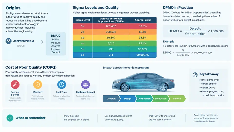
Six Sigma is a disciplined, data-driven methodology for reducing process and product variation to the point where defects become statistically rare. In automotive engineering, it is less a standalone quality program than a shared language that connects design intent, manufacturing capability, supplier performance, and field warranty data. For CAE engineers, Six Sigma provides the statistical framing needed to answer a deceptively simple question: how confident are we that this design will meet its performance targets across the full population of vehicles we will build?
Origins and the Automotive Connection
Six Sigma emerged at Motorola in the mid-1980s as a response to persistent field failures and warranty costs, and was later popularized by General Electric in the 1990s. Its statistical roots, however, trace back to the normal distribution and the work of Walter Shewhart and W. Edwards Deming on statistical process control. The automotive industry adopted it rapidly because vehicle programs already depended on capability studies, gauge R&R, and PPAP-style supplier qualification — Six Sigma gave these activities a unified metric and a structured improvement cycle (DMAIC: Define, Measure, Analyze, Improve, Control).
In a modern vehicle program, Six Sigma thinking appears in several places: tolerance allocation during design, robustness studies in CAE, process capability (Cpk) targets for stamped and cast parts, and the analysis of warranty returns. The methodology's value is that it forces teams to quantify variation rather than argue about nominal values.
Sigma Levels and What They Mean
The "sigma level" of a process expresses how many standard deviations fit between the process mean and the nearest specification limit. A higher sigma level means fewer defects per million opportunities (DPMO). The classic conversion assumes a 1.5σ long-term shift, which accounts for the typical drift of a process over time.
| Sigma level | DPMO (with 1.5σ shift) | Yield | Typical automotive context |
|---|---|---|---|
| 2σ | 308,537 | 69.1% | Manual assembly with weak controls |
| 3σ | 66,807 | 93.3% | Legacy processes, high rework |
| 4σ | 6,210 | 99.38% | Common baseline for many suppliers |
| 5σ | 233 | 99.977% | Mature, well-controlled processes |
| 6σ | 3.4 | 99.99966% | World-class; safety-critical targets |
The DPMO metric normalizes defects by the number of opportunities for a defect, which makes it comparable across processes of different complexity. The formula is:
DPMO = (Number of defects / (Number of units × Opportunities per unit)) × 1,000,000For example, suppose a CAE-supported bracket design is validated against 12 functional requirements, and across a 500-vehicle pilot build, 18 requirement violations are recorded. The DPMO is (18 / (500 × 12)) × 1,000,000 = 3,000. Looking up the sigma table, this corresponds to roughly 4.3σ — a reasonable but not exceptional capability for a structural component.
Cost of Poor Quality in Vehicle Programs
The cost of poor quality (COPQ) is the financial argument for Six Sigma. In automotive programs, COPQ is conventionally split into four categories: internal failure (scrap, rework, re-test), external failure (warranty, recalls, field campaigns), appraisal (inspection, test), and prevention (training, robust design, CAE). The first two are the visible costs; the last two are investments that reduce them.
A useful way to frame this for CAE teams is the "1-10-100 rule": a defect caught in simulation costs roughly 1 unit of effort to fix, in prototype and test 10 units, and in the field 100 units. This is why early robustness studies — DOE, Monte Carlo tolerance analysis, sensitivity studies — carry disproportionate value. A CAE engineer who identifies a 3σ-to-4σ gap in a suspension mount before tooling is released has prevented a cost that would otherwise appear as warranty claims three years later.
How the Concepts Fit Together
The diagram below shows the relationship between the statistical foundation (variation), the metric layer (sigma level, DPMO), the financial layer (COPQ), and the engineering workflow (DMAIC) that connects them. It is a map of the chapter's logic rather than a process flow.
Applying the Framework: A Worked Example
Consider a rear subframe mount whose vertical stiffness must remain within a target window of 42–48 N/mm to satisfy ride and durability requirements. A CAE team runs a Monte Carlo study with 1,000 samples, varying rubber compound modulus (±8%), wall thickness (±0.4 mm), and bushing preload (±5%). The simulated stiffness distribution has a mean of 45.1 N/mm and a standard deviation of 1.3 N/mm.
The distance from the mean to the upper limit is (48 − 45.1) / 1.3 = 2.23σ, and to the lower limit (45.1 − 42) / 1.3 = 2.38σ. The process is therefore limited by the upper side at roughly 2.2σ — well below the 4σ target typical for a safety-relevant mount. Applying the 1.5σ shift, the expected DPMO is on the order of 10,000–20,000, which translates into a meaningful warranty exposure across a production volume of several hundred thousand vehicles.
The Six Sigma response is not to tighten every tolerance. It is to identify which input drives the upper tail — in this case, compound modulus — and to negotiate a tighter incoming material specification or redesign the bushing geometry to reduce sensitivity. That is the Analyze-to-Improve transition, and it is where CAE adds the most value: simulation lets the team test the sensitivity before committing to a tooling change.
Why This Matters for the Rest of the Course
The concepts in this chapter — variation, sigma level, DPMO, and COPQ — are the vocabulary that the remaining DMAIC phases depend on. Define requires a quantified CTQ and a target sigma level. Measure requires a baseline DPMO from simulation or test data. Analyze requires sensitivity and root-cause methods that explain where the variation originates. Improve requires design or process changes validated against the same metric. Control requires monitoring to confirm the sigma level is sustained in production. Without a shared metric, each phase becomes a separate exercise; with it, the program has a single thread from concept to field.