1. Crash CAE optimization landscape

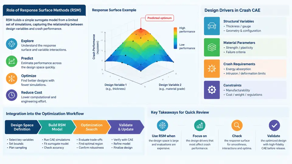
Crashworthiness simulation sits at the most expensive end of the CAE spectrum. A single full-vehicle frontal impact model routinely contains 5–15 million elements, runs for 8–30 hours on a 64–128 core cluster, and produces hundreds of gigabytes of d3plot and time-history output. When a design team needs to explore 40 design variables across a body-in-white (BIW) — gauge thicknesses, material grades, bead depths, joint stiffnesses — the arithmetic is unforgiving: a full-factorial or even a Latin hypercube DOE of 200 runs at 12 hours each is roughly 100 days of wall-clock solver time. Response Surface Methods (RSM) exist precisely to break this cost barrier. Rather than optimizing directly on the solver, RSM builds a cheap mathematical surrogate from a carefully chosen set of simulation runs, then performs the thousands of optimization iterations on that surrogate in seconds.

This chapter establishes the landscape: where RSM fits in a crash CAE optimization workflow, what design drivers dominate crash problems, and how the surrogate integrates with the surrounding toolchain — DOE generation, solver execution, metamodel fitting, optimization, and verification.

Why Crash Problems Resist Direct Optimization

Crash CAE is a poor candidate for gradient-based or direct evolutionary optimization for three structural reasons. First, response non-smoothness: intrusion, acceleration, and force responses are computed from contact and buckling events, so the design space is riddled with discontinuities and local minima. Second, noise: explicit solver outputs vary with time-step, hourglass control, and contact penalty settings, so a 2% change in a response may be numerical rather than physical. Third, cost: each evaluation is expensive enough that population-based methods requiring 10,000 evaluations are infeasible.

RSM addresses all three. A polynomial or Kriging surrogate smooths numerical noise, provides an analytically differentiable (or at least cheaply evaluable) approximation, and reduces the effective evaluation count to the DOE size — typically 30–150 runs for 10–30 variables. The trade-off is approximation error, which must be quantified and controlled through validation runs.

Design Drivers in Crash Optimization

Before selecting a surrogate type, the engineer must understand what is being optimized and how the responses behave. Crash design drivers fall into four families:

• Structural integrity — occupant compartment intrusion (toe pan, dash, A-pillar, door aperture), measured in millimeters against targets such as ≤120 mm toe pan intrusion in a 64 km/h offset deformable barrier (ODB) test.
• Occupant loading — peak acceleration and HIC-derived metrics at the seat track or B-pillar base, typically constrained to ≤ 60–80 g for chest acceleration depending on program targets.
• Energy management — front rail axial crush force, bending resistance, and the balance between crush and bending modes that determines whether the rail folds progressively or collapses.
• Mass and cost — BIW mass, material cost, and manufacturing feasibility (formability, weld access), which act as objectives or constraints alongside the crash responses.

These responses have very different sensitivities and noise levels. Intrusion is relatively smooth and well-behaved; peak acceleration is spiky and sensitive to contact stiffness; mass is exactly computable. A single surrogate type rarely fits all responses equally well, which is why modern workflows fit per-response metamodels and select the type (quadratic polynomial, Kriging, radial basis function) based on cross-validation error.

Where RSM Sits in the Workflow

The diagram below shows the integration of RSM into a crash CAE optimization loop. The key insight is that the surrogate is not a replacement for simulation but a filter: it narrows the design space so that expensive solver runs are spent only on promising candidates and on verification.

The loop has two feedback paths. The first is the infill loop: if verification runs show that the surrogate mispredicts a response by more than an acceptable tolerance (commonly 5–10% for intrusion, 10–15% for acceleration peaks), additional DOE points are added near the Pareto front and the surrogate is refit. The second is the design-space refinement loop: if the optimum sits on a variable bound, the bounds are widened and the process repeats. Both loops are what distinguish a credible RSM study from a one-shot surrogate fit.

Practical Integration Details

In a real toolchain, the handoffs between stages are file-based and scriptable. A typical setup uses a DOE tool (e.g., LS-OPT, modeFRONTIER, or a Python script with pyDOE) to generate a CSV of design variable sets, a batch script to substitute those values into the LS-DYNA keyword deck, and a post-processing script to extract responses from the d3plot or binout. The extraction step is where most integration effort is spent, because crash responses are not single scalars — intrusion must be sampled at specific nodes at specific times, and acceleration must be filtered per SAE J211 before peak extraction.

# Example: response extraction contract (pseudo-code)
responses = {
    "toe_intrusion_mm":  max(node_disp("NODE_TOE", t=0.120)),
    "chest_accel_g":     peak(sae_j211_filter(accel("ACC_CHEST"), cfc=180)),
    "rail_force_kN":     mean(force("XF_Rail"), t=(0.020, 0.060)),
    "biw_mass_kg":       sum(mass(part_set("BIW")))
}
# Each key becomes one surrogate response column in the DOE matrix.

Two integration pitfalls deserve early attention. First, variable parameterization: gauge variables are continuous but manufacturing restricts them to discrete sheet thicknesses (0.6, 0.7, 0.8, 1.0, 1.2 mm, etc.). The surrogate may be fit on continuous variables, but the final candidate must be snapped to a feasible thickness, and the snapped design must be re-verified. Second, response consistency: if the DOE runs use different solver versions or contact settings, the surrogate will absorb that inconsistency as noise. Lock the solver version, time-step control, and hourglass formulation across the entire DOE.

What the Surrogate Buys — and What It Costs

The value proposition is straightforward: a 200-run DOE at 12 hours per run is 100 days of serial solver time, but on a 200-core queue it completes in about 5–7 days. The surrogate fit and a 50,000-evaluation NSGA-II run then take minutes. Verification of 5–10 candidates adds 2–5 days. The total is roughly two weeks versus months for direct optimization — and the Pareto front gives the design team a trade-off map rather than a single point.

The cost is approximation risk. A surrogate that fits the DOE with R² = 0.98 can still mispredict a candidate that lies in an unsampled region, especially for highly nonlinear responses such as rail bending collapse. This is why the verification stage is non-negotiable and why infill strategies (adding points where the surrogate is uncertain) are standard practice. The engineer's job is not to trust the surrogate blindly but to manage its error explicitly — through cross-validation metrics, through verification runs, and through conservative constraint margins during optimization.

With this landscape established, the remaining chapters build the individual competencies: designing the DOE, choosing and validating the surrogate, formulating crash constraints correctly, running the optimizer, and closing the loop with verification.