1. Course overview
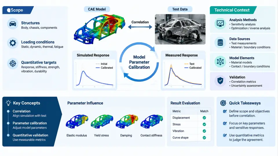
Simulation has become a first-class engineering instrument, but a finite element model is only as trustworthy as the evidence behind it. Quantitative CAE–test correlation is the disciplined practice of comparing simulation output against physical measurement in a way that produces numbers, not impressions: how far apart are the curves, where, in which frequency band, with what uncertainty, and why. Model parameter calibration is the companion activity that adjusts uncertain model inputs — material constants, joint stiffnesses, damping ratios, boundary conditions — so that the model reproduces the measured behavior within an accepted tolerance, while remaining physically defensible.
These two activities form a closed loop. Correlation without calibration tells you the model is wrong but not how to fix it. Calibration without correlation discipline produces a model tuned to one test article, one sensor layout, and one load case — a curve fit masquerading as a predictive model. This course treats them as a single workflow with a shared vocabulary, shared metrics, and shared acceptance criteria.
What "Quantitative" Actually Means
Qualitative correlation — overlaying two plots and declaring them "close" — is where most industrial practice stalls. Quantitative correlation replaces visual judgment with defined metrics and thresholds. Three families of metrics dominate:
- Amplitude metrics — peak-to-peak ratio, RMS ratio, or absolute error at defined reference points, expressed in engineering units or dB.
- Shape metrics — frequency shift of resonant peaks, modal assurance criterion (MAC) between mode shapes, or curve-shape correlation coefficients across a band.
- Statistical metrics — normalized error norms, coefficient of determination, or confidence intervals propagated from measurement uncertainty.
The choice of metric is not cosmetic. A model calibrated to match peak amplitudes may misplace resonances; a model calibrated on MAC alone may match mode shapes while carrying the wrong mass distribution. Mature correlation plans declare the metric set before calibration begins, precisely to prevent metric shopping after the fact.
The Technical Context: Where This Work Sits
Quantitative correlation sits at the intersection of four engineering domains, and the practitioner needs working literacy in each:
| Domain | Contribution to the workflow | Typical failure if neglected |
|---|---|---|
| Test and instrumentation | Measurement uncertainty, sensor placement, excitation and boundary replication | Calibrating the model to measurement artifacts |
| Structural dynamics / mechanics | Mode identification, damping mechanisms, nonlinearity recognition | Forcing a linear model onto nonlinear physics |
| Numerical simulation | Mesh convergence, solver settings, parameter sensitivity | Calibrating discretization error instead of physics |
| Statistics and optimization | Design of experiments, sensitivity ranking, parameter estimation, uncertainty quantification | Non-unique parameter sets, overfitting |
The single most common root cause of failed correlation projects is not a bad optimizer — it is a mismatch between the test boundary conditions and the model boundary conditions. A component tested on soft bungees and modeled as clamped will never correlate, no matter how many parameters are freed. The workflow below makes this visible early.
Scope Boundaries: What This Course Covers and What It Does Not
The course scope is deliberately bounded. It covers structural and mechanical systems — modal, harmonic, transient, and static response — where measurement and simulation can be compared on a common physical basis. It covers parameter calibration for material properties, connection stiffness, damping, and boundary compliance. It covers the statistical machinery needed to make calibration defensible: sensitivity analysis, identifiability checks, regularization, and uncertainty propagation.
It does not attempt to teach finite element theory from first principles, nor transducer physics, nor optimization algorithm internals. Those are prerequisites or adjacent specialisms. The course assumes you can build a reasonable model and run a reasonable test; its value lies in making the two agree for the right reasons.
A Worked Illustration of the Core Idea
Consider a welded bracket assembly. A modal test on a shaker table identifies the first three elastic modes at 142 Hz, 318 Hz, and 507 Hz, with damping ratios of 0.8%, 1.1%, and 1.4%. The initial FE model, using nominal steel properties and rigid tie connections, predicts 151 Hz, 302 Hz, and 540 Hz. The first mode is 6.3% high, the second 5.0% low, the third 6.5% high — a pattern that is not a uniform stiffness scaling, which immediately suggests the error is distributed rather than global.
A sensitivity study on three candidate parameters — weld-zone elastic modulus multiplier, bracket-to-base bolt stiffness, and modal damping — shows that bolt stiffness dominates the first mode (∂f/∂k normalized sensitivity 0.42), weld modulus dominates the third (0.38), and the second mode is comparatively insensitive to both (below 0.12). That insensitivity is a red flag: the second mode's 5% error probably originates in geometry or mass distribution, not in the parameters being calibrated. Freeing bolt stiffness and weld modulus will close the first and third modes but leave the second mode biased — and a practitioner who ignores this will report a "successful" calibration that has absorbed a modeling error into unrelated parameters.
The disciplined response is to fix the model form first — check the bracket's effective mass, verify the weld representation, confirm the test fixture's added mass — then calibrate. After correcting a 0.6 kg instrumentation mass omission in the model, the second mode moves to 314 Hz, and the subsequent two-parameter calibration converges to 143 Hz, 316 Hz, and 509 Hz, all within 1.5% of test. Validation on a separate impact-hammer dataset at a different excitation point confirms the updated model predicts the first mode within 1.2% — evidence that the calibration captured physics rather than fitting one dataset.
Prerequisites and Working Assumptions
To get full value from this course, you should be comfortable with: linear structural dynamics (modal superposition, frequency response functions), basic statistics (means, variances, regression, confidence intervals), and at least one commercial FE environment (Nastran, Abaqus, ANSYS, or equivalent). Familiarity with a scripting environment — Python with NumPy/SciPy is the assumed default — is strongly recommended, because serious calibration work is scripted, versioned, and reproducible, not clicked through a GUI.
One convention is fixed for the entire course and should be noted now: frequency errors are reported as (f_sim − f_test)/f_test × 100%, so a positive value means the model over-predicts frequency. Amplitude errors are reported in dB as 20·log₁₀(A_sim/A_test). All correlation tables and figures follow this sign convention unless explicitly stated otherwise.
What You Will Be Able to Do
By the end of the course you will be able to design a correlation plan before running either test or simulation; compute and interpret a defensible metric set; rank parameters by sensitivity and screen out non-identifiable ones; execute a bounded calibration that respects physical limits; quantify the uncertainty in the calibrated parameters; and validate the result on data the calibration never saw. Those five capabilities, taken together, are what separates a model that can support a design decision from a model that merely produces colorful plots.