1. Course overview

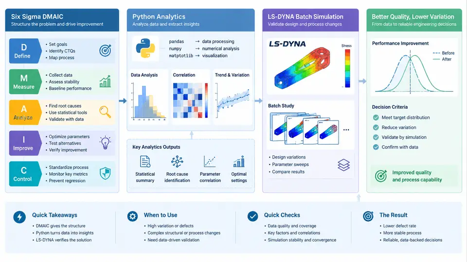
Engineering quality improvement rarely fails because a team lacks simulation capability. It fails because simulation output is disconnected from a disciplined improvement method, and because the analysis of that output is manual, inconsistent, and impossible to audit. This course addresses both gaps at once: it teaches you to run the Six Sigma DMAIC loop with Python as the analytical engine and LS-DYNA as the physics engine, so that every simulation run, every extracted metric, and every statistical conclusion is traceable to a defined question and a reproducible script.

The three components play distinct roles. DMAIC (Define, Measure, Analyze, Improve, Control) supplies the problem-solving structure and the statistical rigor — it forces you to state a measurable response, establish a baseline, prove that a factor actually matters, and lock in the gain. LS-DYNA supplies the physics: explicit dynamic simulation of impact, crash, drop, penetration, and other transient events where the response of interest (peak acceleration, intrusion, energy absorption, plastic strain) cannot be measured cheaply or safely on hardware. Python is the connective tissue: it parameterizes the input decks, launches and monitors batch runs, parses the binary and text output, computes the response metrics, and feeds them into the statistical models that DMAIC requires.

Why batch simulation, not single runs

A single LS-DYNA run answers "what happens for this design." Six Sigma asks "which factors move the response, by how much, and with what confidence." Answering that requires a designed set of runs — a DOE matrix, a tolerance sensitivity sweep, or a Monte Carlo sample — executed consistently and analyzed as a population. Manual execution does not scale: a 32-run fractional factorial with three replications is 96 jobs, each producing a d3plot, nodout, glstat, and rcforc file that must be reduced to a handful of numbers. The batch layer is what makes the statistical layer possible.

The end-to-end architecture

The diagram below shows how the three components interlock across a single DMAIC cycle. Note that the Python layer appears twice — once upstream to generate and launch cases, once downstream to reduce results and fit models — and that the Control phase feeds parameters back into the case generator, closing the loop.

What a working cycle looks like

Consider a representative problem: a handheld device must survive a 1.2 m drop onto concrete without the internal bracket exceeding a peak acceleration of 1500 g at the PCB mounting boss. In Define, the response Y is peak acceleration at a named node set; the CTQ limit is 1500 g; the factors under study are bracket thickness (1.2–2.0 mm), rib count (0–4), and corner fillet radius (0.5–2.0 mm). In Measure, you establish the baseline by running the nominal design and confirming that the metric extraction is repeatable — running the identical deck twice should return peak acceleration within a fraction of a percent, and if it does not, the extraction window or the filtering is wrong, not the physics.

In Analyze, a two-level, three-factor design with a center point (nine runs) is generated by the Python case generator, which substitutes the factor values into a parameterized keyword template. Each deck is launched, monitored for normal termination, and reduced to a single row. A regression on coded factors then reveals which terms are significant. Suppose the fit returns bracket thickness as dominant, rib count as secondary, and a thickness × rib interaction that is significant at p < 0.05 — that interaction is the finding a one-factor-at-a-time study would have missed entirely.

In Improve, the fitted model is used to predict the setting that minimizes peak acceleration while respecting mass and manufacturability constraints, and a confirmation run at that setting verifies the prediction falls inside its confidence interval. In Control, the validated parameter set is frozen into the released deck, and a control chart on subsequent re-validation runs (or on production drop-test data) monitors whether the response drifts outside the established limits.

Prerequisites and the working environment

You should be comfortable with basic statistics (mean, variance, hypothesis testing) and have seen an LS-DYNA keyword deck before. The Python stack is deliberately conventional: pandas for tabular assembly, numpy for array work, statsmodels for regression and ANOVA, scipy for distributions, and matplotlib for the plots that go into the report. For LS-DYNA output parsing, the course uses lasso-python where available and plain text parsing of glstat and nodout where it is not, so the workflow does not depend on a single vendor library.

Common failure modes this course teaches you to catch

Three problems account for most wasted effort in simulation-driven Six Sigma work. First, silent solver failures: a run that terminates with a negative volume or an energy error still writes output files, and a naive reducer will happily extract a peak acceleration from a physically meaningless result. The batch layer must record termination status and energy ratio alongside every metric, and the analytics layer must exclude flagged runs before fitting. Second, metric definition drift: if the node set or the filter used to compute peak acceleration changes between the baseline and the confirmation run, the comparison is void. The extraction script must be version-controlled and referenced by hash in the results table. Third, over-fitting the DOE: with nine runs and a three-term model, the residual degrees of freedom are thin, and a high R² can be an artifact. The course consistently pairs model fit with a confirmation run rather than trusting the regression alone.

How the thirty chapters are organized

The course moves from foundations to a complete worked cycle. Early chapters establish the DMAIC framing, the Python environment, and the structure of an LS-DYNA deck that can be parameterized. The middle chapters build the batch infrastructure — case generation, job scheduling, status monitoring, and robust output reduction — and then the statistical layer on top of it: response tables, simulation MSA, ANOVA, regression, and response surface methods. Later chapters cover optimization under constraints, confirmation runs, control charting, and the reporting and handover artifacts that make the result usable by someone who did not run the study. Each chapter produces a concrete artifact — a script, a template, a results table, or a report section — that accumulates into a complete, reproducible DMAIC case study by the end.

The through-line is simple: define the question statistically, answer it with physics, and let Python hold the two together so that the answer is both defensible and repeatable.