1. Measurement system analysis in CAE valid
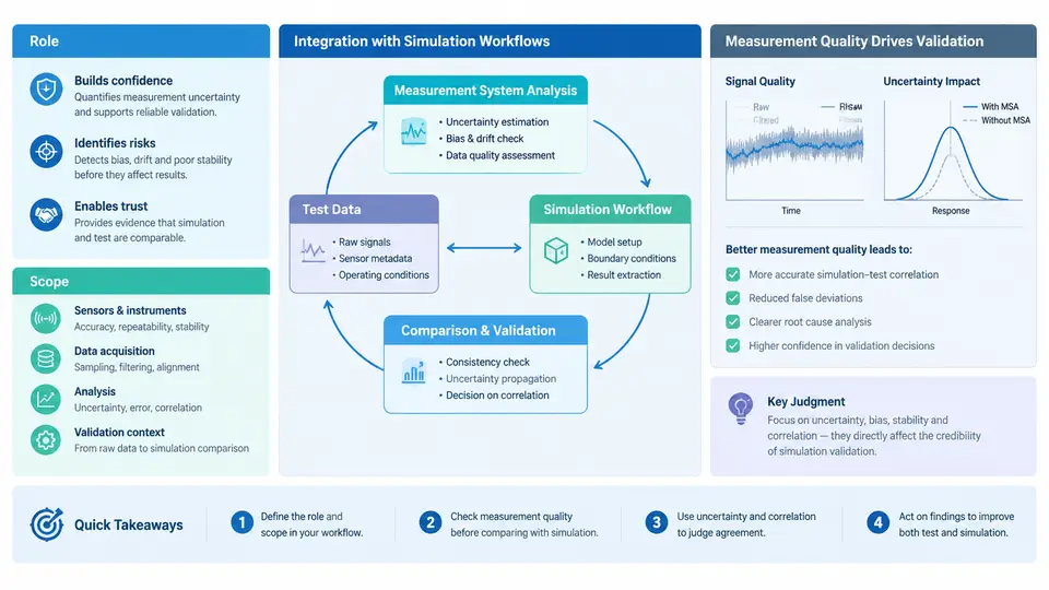
In physical testing, measurement system analysis (MSA) is a familiar discipline: before trusting a strain gauge reading or a load cell output, we quantify repeatability, reproducibility, bias, linearity, and stability. In CAE validation, the "measurement system" is not a single instrument but an entire chain — solver, discretization, material model, boundary conditions, post-processing extraction, and the comparison metric itself. Treating that chain as a measurement system, and applying MSA logic to it, is what separates a defensible validation from a plausible-looking correlation plot.
This chapter establishes the role and scope of MSA within CAE validation and shows how it integrates with the simulation workflow. The goal is not to import physical-metrology paperwork wholesale, but to adopt its core discipline: separate the variation you care about from the variation introduced by how you measured it, and quantify both before drawing conclusions.
Why CAE Validation Needs Its Own MSA
A validation statement such as "the model predicts peak stress within 8% of test" is only meaningful if both sides of that comparison are characterized. The test side has a measurement system with known uncertainty. The simulation side has a numerical measurement system whose uncertainty is rarely quantified and often assumed to be negligible. In practice, it is frequently not negligible: mesh density, element formulation, contact stiffness, time-step size, and extraction location can each shift a reported peak by several percent — the same order as the correlation error being claimed.
Consider a representative example. A bracket is instrumented with rosette strain gauges, and a linear static simulation is run for the same load case. The reported correlation error at the critical location is 12%. Before concluding the material model is wrong, an MSA-minded engineer asks: how repeatable is the gauge installation and readout (±3% at 95% confidence)? How sensitive is the simulated strain to mesh refinement at that fillet (a convergence study shows 4% change between the medium and fine mesh)? How much does the extraction point move if the gauge is placed 2 mm off nominal (a placement-sensitivity run shows 5%)? Combined, the measurement-side uncertainty can plausibly account for a large fraction of the 12%. The validation conclusion changes from "model is inaccurate" to "model is within combined measurement uncertainty at this location" — a materially different engineering statement.
Scope: What Counts as the Measurement System
For CAE validation, define the measurement system as the complete path from physical excitation to the compared quantity. A practical scoping checklist covers four layers:
- Physical acquisition layer — sensors, calibration status, DAQ resolution, sampling rate, filtering, and mounting effects (e.g., gauge bonding, accelerometer mass loading).
- Test data reduction layer — channel scaling, zeroing, outlier removal, averaging windows, and derivation of quantities such as principal strain or modal damping.
- Numerical measurement layer — mesh and element type, solver tolerances, contact and nonlinear settings, boundary condition idealization, and the extraction method (nodal vs. elemental, averaging, probe location).
- Comparison layer — the metric itself: pointwise error, RMS deviation, MAC for mode shapes, peak-to-peak ratio, or frequency shift, together with its tolerance band.
Scope decisions should be driven by the validation question. A modal correlation study needs tight control over sensor mass loading and mode-extraction settings; a static strength correlation needs tight control over gauge placement and mesh convergence at the hot spot. Applying full rigor everywhere is wasteful; applying none is indefensible.
Integration with the Simulation Workflow
MSA is not a post-hoc audit performed after the correlation plot is produced. It integrates at three points in the workflow, and the figure below shows how the numerical measurement system and the physical measurement system converge on a single comparison with an explicit uncertainty budget.
Before simulation. The validation plan fixes the comparison metric and its acceptance tolerance, and derives a preliminary uncertainty budget. This determines mesh targets, extraction conventions, and sensor placement — for example, specifying that the simulated strain be extracted as a nodal average over a 5 mm patch to match the gauge grid area, rather than as a single nodal peak.
During simulation. Numerical MSA runs are executed as part of the study, not as an afterthought: a mesh convergence study at the extraction location, a boundary-condition sensitivity run (e.g., varying bolt preload or contact stiffness by a realistic range), and a solver-tolerance check. Each produces a contribution to u_num.
At comparison. The measured and simulated quantities are compared together with their combined uncertainty. The decision rule is explicit: if the observed deviation falls within the combined uncertainty band, the model is consistent with the test at that location; if it exceeds the band, the excess is a candidate model-form error worth investigating.
A Worked Uncertainty Budget
The following table is an illustrative budget for the bracket example above. Values are representative assumptions for teaching purposes, not measured results.
| Source | Layer | Estimated contribution (95%) | Basis |
|---|---|---|---|
| Gauge installation & readout | Physical | ±3.0% | Repeated installs, GR&R |
| Gauge placement tolerance | Physical | ±5.0% | Placement-sensitivity run |
| Mesh convergence at fillet | Numerical | ±4.0% | Medium vs. fine mesh |
| Contact stiffness range | Numerical | ±2.5% | Parameter sweep |
| Extraction convention | Numerical | ±1.5% | Nodal vs. patch average |
Combining in quadrature (assuming independence, a simplifying assumption to be stated explicitly): u_comb = √(3.0² + 5.0² + 4.0² + 2.5² + 1.5²) ≈ 7.8%. The observed 12% deviation exceeds this band, so roughly 4 percentage points remain unexplained and justify a model investigation — but the investigation now starts from a quantified baseline rather than a bare number.
Practical Integration Points and Failure Symptoms
Three integration failures recur in practice. First, metric drift: the comparison metric is redefined after results are seen (switching from peak to average to improve agreement). Prevent this by freezing the metric and tolerance in the validation plan. Second, hidden numerical variation: different analysts extract the same quantity differently, producing scatter that masquerades as model error — the numerical analogue of appraiser variation. Mitigate with a written extraction convention and a reproducibility check where two analysts process the same result files. Third, uncalibrated acceptance: tolerances set by convention ("within 10%") rather than derived from the uncertainty budget, which can make a good model fail or a poor one pass.
The deliverable of this integration is a validation record in which every compared quantity carries its uncertainty budget, its basis, and its owner. That record is what allows a reviewer to distinguish a genuine model deficiency from measurement noise — and it is the foundation on which the remaining chapters of this course build, from GR&R for test data through numerical sensitivity methods to the statistical decision rules used at the comparison stage.