1. Crash CAE workflow and uncertainty sourc
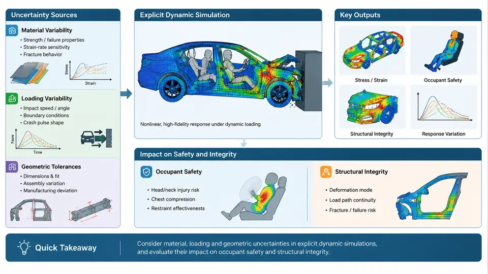
Crash CAE is the numerical backbone of modern occupant-safety and structural-integrity development. Before any DOE, surrogate model, or uncertainty-quantification (UQ) study can be meaningful, the analyst must understand what the explicit-dynamic workflow actually computes, where variability enters that workflow, and how each source propagates into the safety metrics that engineers ultimately judge. This chapter establishes that foundation: it maps the standard crash simulation chain, classifies the dominant uncertainty sources, and shows how small input perturbations translate into measurable changes in occupant injury criteria and structural response.
The explicit dynamic simulation chain
A frontal or side impact event lasts roughly 80–150 ms. Because the physics is dominated by inertia, contact, and large deformation, crash CAE uses an explicit time-integration solver (for example LS-DYNA, Radioss, or Abaqus/Explicit). The central-difference scheme advances the solution at a stable time step governed by the smallest element and the material wave speed:
Δt_crit ≈ L_min / c,   c = sqrt(E / ρ)
# Example: L_min = 4 mm steel element
# E = 210 GPa, ρ = 7850 kg/m³  →  c ≈ 5170 m/s
# Δt_crit ≈ 4e-3 / 5170 ≈ 0.77 µs  (before mass scaling)
The workflow proceeds through a fixed sequence of modelling decisions, each of which introduces its own assumptions:
- Geometry preparation — CAD cleanup, mid-surface extraction for thin-walled parts, and mesh generation. Shell elements dominate the body-in-white (BIW); solid elements appear in castings and closures.
- Material and connection definition — elastic-plastic metals with strain-rate sensitivity (e.g., Johnson–Cook or *MAT_024 with rate curves), spot welds, adhesives, and bolted joints.
- Boundary and initial conditions — prescribed rigid-barrier velocity (e.g., 50 km/h frontal, 32 km/h side pole), gravity, and contact definitions.
- Occupant and restraint modelling — Hybrid III or THOR dummy FE models, airbags, seat belts with pretensioners and load limiters.
- Solution and post-processing — energy-balance checks, intrusion measurement, and injury-criterion extraction.
The output metrics that matter are well defined: Head Injury Criterion (HIC), chest deflection and viscous criterion (VC), femur and tibia loads, plus structural measures such as B-pillar intrusion, toe-pan intrusion, and peak deceleration at the seat track. These are the quantities that DOE and UQ will later treat as responses.
Where uncertainty enters
No single simulation is deterministic in practice. Variability enters from four broad families, and understanding their relative magnitude is what makes a UQ study efficient rather than exhaustive.
Material variability. Sheet-steel yield strength in production coils typically scatters with a coefficient of variation (CoV) of 3–8%; high-strength grades and aluminium castings can exceed 10%. Strain-rate parameters and failure strains are even less certain because they are extrapolated from coupon tests at limited rates. A 5% shift in yield stress on a front rail can change the crash pulse and, through it, the occupant deceleration history.
Loading variability. Barrier speed, impact angle, and offset are never exactly nominal. Regulatory corridors allow tolerances (e.g., ±1 km/h on impact speed, small yaw offsets), and real-world crashes span a wide distribution. Loading uncertainty often dominates the response variance because crash response is highly nonlinear near buckling and fracture thresholds.
Geometric tolerances. Stamping springback, weld-position scatter, and assembly gap variation shift section properties and trigger points. A 2 mm offset in a crush initiator or a 1° change in a longitudinal's bend angle can flip a deformation mode from stable folding to global bending — a discontinuous, high-consequence effect.
Modelling and numerical uncertainty. Mesh size, hourglass control, contact stiffness, and mass scaling are analyst choices, not physical variability. They belong to a separate epistemic category and should be handled through verification and sensitivity studies rather than sampled as random variables.
How variability propagates to safety metrics
The figure below traces the causal chain from input scatter to the two outcome families — occupant safety and structural integrity — and highlights the nonlinear "mode-switch" region where small inputs produce large response jumps.
Two features of this chain deserve emphasis. First, the mapping from inputs to outputs is strongly nonlinear and non-monotonic: intrusion may be nearly flat to a 3% yield-strength change, then jump sharply once a rail passes its buckling threshold. Second, the two outcome families are coupled — a stiffer front structure reduces intrusion (good for integrity) but can raise occupant deceleration (bad for HIC). A UQ study that optimizes one metric in isolation will mislead design.
A worked sensitivity illustration
Consider a simplified frontal model with three uncertain inputs: front-rail yield stress (lognormal, mean 620 MPa, CoV 5%), impact speed (normal, 50 km/h, σ = 0.5 km/h), and crush-initiator position offset (uniform, ±2 mm). A screening run of 30 Latin-hypercube samples is enough to rank influence before committing to a full DOE. The expected observations — clearly illustrative, not measured — are typically:
| Input | Distribution | Dominant effect | Typical ranking |
|---|---|---|---|
| Impact speed | N(50, 0.5) km/h | Scales total kinetic energy; shifts whole pulse | 1 (largest on HIC) |
| Yield stress | LN(620, 5%) MPa | Changes crush force and folding mode | 2 (largest on intrusion) |
| Initiator offset | U(−2, +2) mm | Triggers mode switch near threshold | 3 on average, but high tail risk |
The practical lesson: rank by both mean effect and tail effect. The initiator offset may look minor in a mean-based ranking yet dominate the 95th-percentile intrusion because it controls whether a rail folds stably or bends globally. This is precisely why the course moves from workflow and source identification into DOE design and then into distribution-aware UQ.
Verification before quantification
Before any sampling campaign, confirm the baseline model is trustworthy. Check that hourglass energy stays below roughly 5% of internal energy, that added-mass from scaling is under ~1–2% and does not alter the pulse, and that total energy is conserved (kinetic converts to internal plus contact energy with no unexplained growth). A model that fails these checks will produce a response surface that reflects numerical artefacts rather than physics, and no amount of sophisticated DOE will recover the lost credibility.
With a verified baseline, a clear map of aleatory sources, and an explicit separation of epistemic choices, the analyst is ready to design experiments that sample the right variables at the right resolution — the subject of the next stage of the workflow.