1. Occupant CAE response landscape
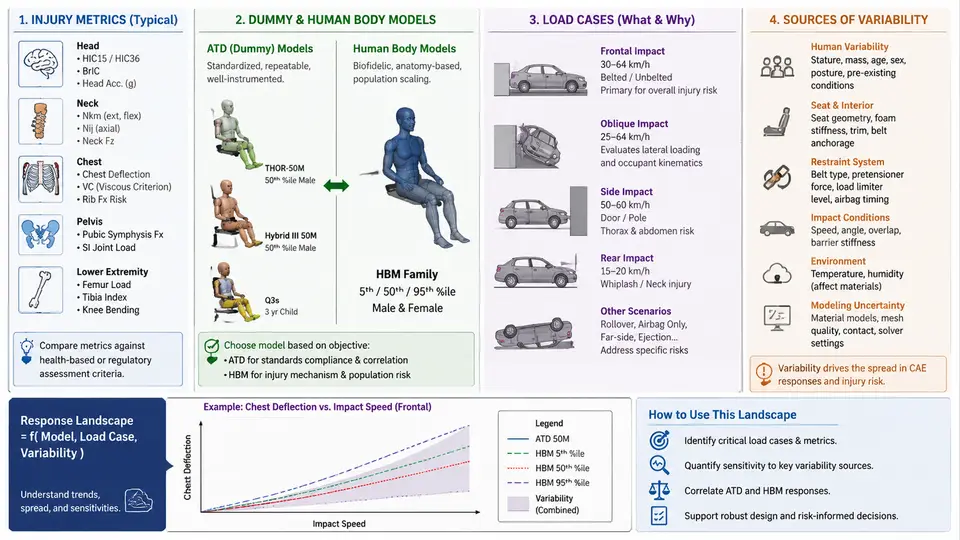
Occupant CAE is the discipline of predicting how a human body responds to a crash environment before any physical test is run. Its outputs feed restraint design, vehicle structure tuning, and regulatory compliance arguments. Before any correlation or regression work makes sense, you need a clear mental map of what is being predicted (injury metrics), what is doing the predicting (dummy and human body models), what conditions drive the prediction (load cases), and where the scatter comes from (variability). This chapter builds that map and establishes the vocabulary used throughout the course.
Injury metrics: the response quantities we correlate
CAE does not predict "injury" directly; it predicts physical channels — accelerations, forces, moments, deflections, pressures — from which injury criteria are computed. The most common families are:
- Head: HIC15/HIC36 from the resultant translational acceleration at the head CG, rotational criteria such as BrIC (from peak angular velocity components) and DAMAGE/CSDM-style metrics for brain tissue, plus linear/rotational acceleration limits in regulations.
- Neck: Nij (combined axial force and bending moment, normalized by intercept values), shear force, and extension/flexion moments.
- Chest: chest deflection (absolute or normalized to half-chest depth), chest acceleration (3 ms clip), and the Viscous Criterion VC = 1.3·v(t)·C(t).
- Abdomen and pelvis: belt force, penetration, and pubic symphysis force/deflection depending on the model.
- Lower extremities: femur axial force, tibia index, and knee-thigh-hip loading.
Two practical points matter for correlation work. First, criteria are derived quantities: a small phase error in an acceleration trace can shift HIC noticeably, so correlation targets should be defined at the channel level (acceleration time history) as well as at the criterion level. Second, criteria are filtered and windowed (e.g., CFC 1000 for HIC, CFC 600 for chest acceleration). Always record the filter class and window used, because comparing an unfiltered CAE signal to a filtered test signal is a classic source of false disagreement.
Dummy and human body models
Two model families dominate. Anthropomorphic test devices (ATDs) — Hybrid III 50th percentile male, THOR-50M, Hybrid III 5th percentile female, Q-series child dummies, WorldSID and ES-2re for side impact — are calibrated, durable, and legally referenced. Their CAE counterparts are validated against the physical dummy's certification corridors, so they are the natural choice when the correlation target is a sled or vehicle test with a dummy. Human body models (HBMs) — GHBMC, THUMS, and similar — represent anatomy with deformable organs and are used for injury prediction beyond dummy measurement capability, parameter studies, and restraint optimization. They are not certified devices, so their correlation targets are usually cadaver or PMHS tests, volunteer data, or field reconstruction.
The choice of model changes the correlation problem. Dummy models are stiff, nonlinear, and dominated by contact and joint friction; HBM responses are softer, more sensitive to material properties and mesh, and often show greater run-to-run and model-to-model scatter. A regression fitted on Hybrid III chest deflection will not transfer to an HBM chest deflection without re-derivation.
Load cases and the test matrix
Occupant CAE load cases fall into a few families: frontal full-width and offset deformable barrier (ODB), frontal sled with pulse input, side impact (MDB and pole), rear impact, and rollover. Each family has a characteristic input (barrier impact speed, sled pulse, pole angle) and a characteristic occupant response. Within a family, the matrix is expanded by seating position, restraint configuration (belt only, belt plus pretensioner and load limiter, airbag variants), occupant size, and impact angle.
For correlation, the load case must be reproduced at the level of the input boundary condition, not just the nominal test name. A frontal sled correlation requires the measured sled pulse (acceleration vs. time, with its filter class), the belt geometry and anchor positions, the seat cushion stiffness, and the airbag firing time and inflator output. If any of these differ between test and CAE, the residual will contain a systematic bias that no regression can remove.
Sources of variability
Variability enters from four directions, and separating them is the core diagnostic skill of this course:
- Test variability: pulse shape differences between runs, belt routing and pretensioner timing, dummy positioning and joint settling, sensor mounting, and measurement noise. Repeat tests on the same configuration typically show a few percent scatter in peak chest deflection and larger scatter in HIC.
- Model variability: mesh density, material card calibration, contact definitions, hourglass control, and solver settings. Two teams modeling the same dummy can produce different peak responses.
- Parameter variability: friction coefficients, belt stiffness, airbag mass flow, and occupant anthropometry. These are the inputs a regression model is usually built to capture.
- Boundary variability: how the pulse, seat, and restraint are represented. This is often the largest single contributor and the easiest to overlook.
Why this landscape matters for correlation and regression
Every regression model in this course is a statement of the form "response = f(parameters) + error." The landscape above tells you what belongs on each side. The response side is a filtered channel or a derived criterion, tied to a specific model and load case. The parameter side is the set of inputs you are willing to vary — belt stiffness, friction, airbag mass flow, occupant size — and the error term absorbs everything you chose not to model, including boundary and model variability. If the error term is dominated by boundary mismatch, the fitted coefficients will look precise but will not generalize.
A concrete example makes the point. Suppose you are correlating Hybrid III 50th percentile chest deflection in a 40 km/h frontal sled. You have five repeat tests and five CAE runs with the same nominal inputs. If the test peak deflections range from 32 to 36 mm and the CAE peaks range from 30 to 39 mm, the CAE scatter is larger than the test scatter. Before building a regression of deflection on belt stiffness, you should first reduce the CAE scatter by checking contact definitions, hourglass energy, and belt element formulation. Only when CAE repeatability is comparable to test repeatability does a regression on physical parameters become meaningful.
What to carry forward
Keep four things explicit in every study: the injury metric definition (channel, filter, window), the model identity and version (dummy model release or HBM version), the load case boundary conditions (pulse, restraint, seat), and the variability budget (test, model, parameter, boundary). These four items form the metadata that makes a regression result interpretable and reproducible. The next chapters build the statistical machinery on top of this foundation, starting with how to characterize and compare response signals before any model is fitted.