1. Multi-solver automotive simulation lands
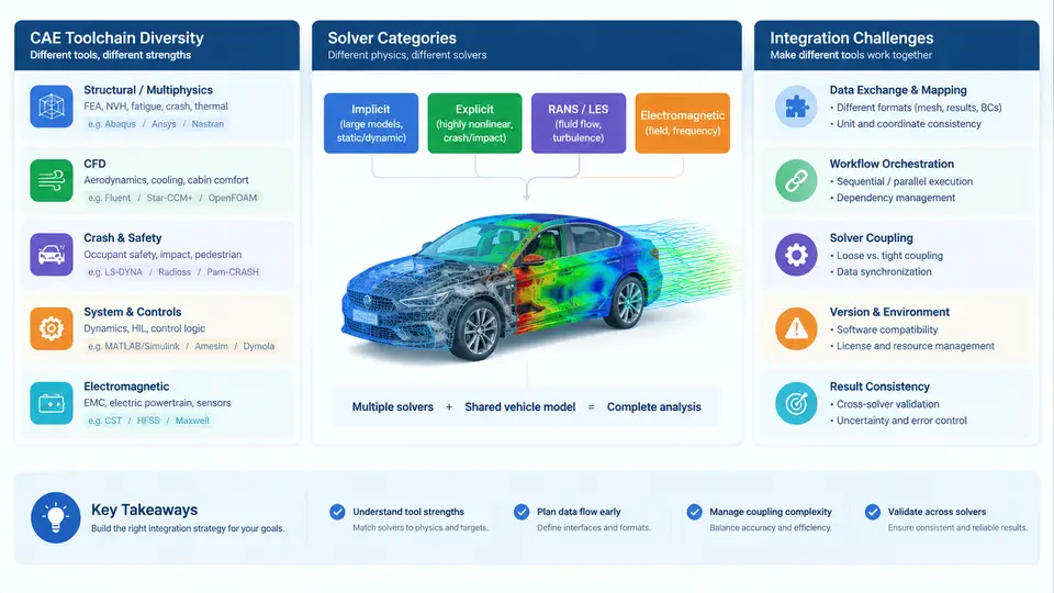
Modern vehicle development is no longer a single-tool discipline. A typical OEM or Tier-1 engineering organization runs dozens of simulation codes simultaneously, each chosen because it solves a specific class of physics better than its neighbors. Understanding this landscape — which solver categories exist, why the toolchain is so diverse, and where integration breaks down — is the prerequisite for any integration management strategy.
Why the Toolchain Is Inherently Diverse
Vehicle programs must answer questions across radically different physical regimes and time scales. A crash event resolves in roughly 100–150 ms but requires explicit time integration with microsecond steps. A powertrain thermal soak can span hours and is best handled implicitly. Aerodynamic drag optimization needs steady-state CFD on meshes of 200–500 million cells. NVH analysis operates in the frequency domain. No single numerical method covers this range efficiently, so the industry standardized on specialized solvers and accepted the integration cost as a necessary trade-off.
Three structural forces drive diversity further:
- Physics fidelity requirements — crash, durability, and safety certification demand explicit structural codes with proven material models and regulatory validation histories.
- Legacy and supply-chain inertia — Tier-1 suppliers deliver subsystem models in their own native formats, and OEMs must ingest them rather than dictate a single tool.
- Vendor specialization — commercial vendors optimize for specific domains (e.g., LS-DYNA for crash, Fluent/STAR-CCM+ for CFD, Adams for multibody dynamics), and no vendor dominates all domains.
Solver Categories in Vehicle Development
The table below summarizes the major solver categories, their dominant numerical approaches, and representative tools encountered in automotive CAE integration work.
| Category | Numerical Approach | Typical Tools | Primary Vehicle Applications |
|---|---|---|---|
| Explicit structural (crash) | Explicit time integration, penalty contact | LS-DYNA, Radioss, Abaqus/Explicit | Frontal/side impact, occupant restraint, pedestrian protection |
| Implicit structural (strength/durability) | Implicit Newton–Raphson, direct/sparse solvers | Abaqus/Standard, Nastran, OptiStruct | Body stiffness, fatigue life, modal analysis |
| CFD (external/internal) | Finite volume, RANS/LES turbulence models | Fluent, STAR-CCM+, OpenFOAM | Aerodynamics, underhood thermal, HVAC duct flow |
| Multibody dynamics (MBD) | Rigid/flexible body equations of motion | Adams, Simpack, MotionSolve | Suspension kinematics, ride comfort, load prediction |
| 1D system simulation | Lumped-parameter ODE/DAE networks | AMESim, GT-SUITE, Simulink | Powertrain thermal, hydraulic circuits, energy management |
| NVH / acoustics | FEM/BEM frequency response, SEA | Nastran, Actran, VA One | Structure-borne noise, airborne transfer, panel vibration |
| Electromagnetics | FEM/FDTD, method of moments | Maxwell, CST, FEKO | E-motor design, EMC/EMI, antenna placement |
Each category carries its own mesh conventions, material model libraries, unit systems, and result formats. A crash model may use millimeter–tonne–second units with a fully integrated shell mesh, while a CFD model uses meters with polyhedral cells and turbulence wall functions. These are not cosmetic differences; they determine what data can be exchanged and at what fidelity.
Integration Challenges Across the Toolchain
Integration problems in multi-solver environments fall into four recurring classes:
- Geometry and mesh mismatch. A body-in-white CAD assembly may be meshed independently for crash (coarse shell, ~5 mm target) and NVH (finer shell, ~3 mm). Mapping loads or displacements between dissimilar meshes introduces interpolation error that can reach 10–20% in local stress hotspots if not controlled.
- Data format and unit incompatibility. Solver A exports nodal forces in N and mm; Solver B expects kN and m. Without a governed conversion layer, silent unit errors propagate through co-simulation and produce plausible but wrong results.
- Time-step and coupling mismatch. Co-simulation between an explicit crash solver (µs steps) and a 1D thermal network (ms steps) requires a coupling scheme that neither destabilizes the explicit side nor starves the implicit side of information.
- Version and configuration drift. When the CAD geometry changes, every downstream mesh, material assignment, and boundary condition must be re-validated. Without traceability, teams lose track of which solver model corresponds to which design freeze.
Visualizing the Integration Landscape
The diagram below maps the major solver categories, their data exchange paths, and the integration friction points that arise at each interface. It is intended as a reference map for the rest of this course.
What Integration Management Must Deliver
Given this landscape, integration management is not a single tool or file format. It is a governed set of practices that ensures: (1) geometry and mesh data can be exchanged with quantified and acceptable interpolation error; (2) units and coordinate systems are explicitly declared and validated at every interface; (3) coupling schemes are stable and their time-step ratios are documented; and (4) every solver model is traceable to a specific design revision and boundary-condition set.
The chapters that follow will address each of these areas in detail — from mesh mapping algorithms and unit governance to co-simulation orchestration and configuration management. The goal is not to eliminate solver diversity, which is technically necessary, but to make the interfaces between solvers predictable, auditable, and reproducible.