1. Crash safety prediction landscape
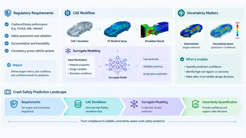
Crash safety prediction sits at the intersection of regulatory compliance, physics-based simulation, and statistical inference. Before any surrogate model or uncertainty-aware framework can be justified, it is worth mapping the landscape: what regulations demand, how CAE workflows actually operate, where surrogate models enter the picture, and why uncertainty quantification (UQ) is no longer optional.
Regulatory Requirements: The Compliance Backbone
Vehicle crash safety is governed by a layered set of standards. In the United States, FMVSS 208 (occupant crash protection) and FMVSS 214 (side impact) define pass/fail criteria based on measured injury metrics — HIC (Head Injury Criterion), chest deflection, femur axial force, and Nij (neck injury criterion). In Europe, UNECE R94/R95 and the Euro NCAP consumer rating protocol impose overlapping but not identical requirements. China's GB 11551 and C-NCAP add another regulatory surface.
These regulations share a critical characteristic: they are deterministic pass/fail thresholds applied to stochastic physical events. A vehicle must not exceed HIC 700 in a 56 km/h frontal rigid barrier test, but the actual HIC value depends on manufacturing tolerances, material property scatter, occupant positioning, and sensor placement. The regulation does not ask "what is the probability of exceeding HIC 700?" — it asks "did this specific test exceed it?" This gap between deterministic regulation and stochastic reality is precisely where UQ becomes essential.
The CAE Workflow: From CAD to Injury Metrics
A typical crashworthiness CAE workflow proceeds through several stages, each introducing its own uncertainty sources:
- Geometry preparation: CAD models are cleaned, meshed (typically 5–8 mm shell elements for body structure, 10–20 mm for occupant regions), and assembled into a full vehicle model. Mesh quality variation alone can shift peak acceleration by 3–8%.
- Material modeling: Steel grades (DP590, DP780, boron steel) require calibrated Johnson-Cook or GISSMO damage models. Tensile test scatter of ±5% in yield strength propagates directly into crash pulse variation.
- Boundary and initial conditions: Barrier alignment, impact angle, velocity (typically 50–64 km/h), and occupant posture (Hybrid III 50th percentile, THOR, or Human Body Model) are specified. Real-world variation in these parameters is substantial.
- Solver execution: Explicit finite element solvers (LS-DYNA, PAM-CRASH, Radioss) integrate the equations of motion. A single full-vehicle frontal impact model may contain 5–15 million elements and require 12–48 hours on 64–256 CPU cores.
- Post-processing: Acceleration-time histories are filtered (SAE J211 CFC 60 or 180), and injury criteria are computed. The choice of filter class and time window can alter HIC by 5–15%.
The computational cost is the central bottleneck. A design-of-experiments (DOE) study with 50 variables and 5 levels each would require 550 simulations — computationally impossible. Even a modest 20-run Latin Hypercube sample at 24 hours per run consumes 480 CPU-hours per design iteration.
Surrogate Modeling: The Computational Bridge
Surrogate models — also called metamodels or response surfaces — replace the expensive FE solver with a cheap mathematical approximation. Common choices include:
- Polynomial response surfaces: Fast to fit, but poor for highly nonlinear crash responses.
- Kriging / Gaussian Process regression: Provides both a prediction and a variance estimate, making it naturally suited for UQ. However, fitting scales as O(n³) in the number of training points.
- Radial Basis Functions (RBF): Good for scattered data, but no inherent uncertainty estimate.
- Neural networks / Deep learning: Capable of handling high-dimensional inputs, but require large training sets and provide no native uncertainty quantification unless combined with Bayesian methods or ensembles.
The surrogate model's role is to enable rapid exploration of the design space: sensitivity analysis, optimization, and reliability assessment. But a surrogate without uncertainty bounds is a point estimate masquerading as knowledge.
Why Uncertainty Quantification Matters
UQ in crash safety serves three distinct purposes:
1. Design robustness. A design that passes HIC 700 in nominal simulation may fail in 30% of production vehicles due to manufacturing scatter. UQ quantifies this risk, enabling robust design optimization that accounts for parameter variability.
2. Model validation. Comparing simulation to physical test requires acknowledging that both sides have uncertainty. A validation metric that ignores test scatter and solver error is not a validation metric — it is a comparison of two point estimates.
3. Regulatory margin setting. If a manufacturer knows that HIC has a standard deviation of 40 across the production population, they can set a nominal design target of HIC 600 to ensure a 99.7% compliance rate (assuming normality). Without UQ, this margin is set by engineering judgment alone.
Visualizing the Landscape
The following diagram maps the relationships between regulatory requirements, CAE workflow stages, uncertainty sources, and the role of surrogate modeling with UQ. It is not a linear process flow; rather, it shows how uncertainty enters at multiple points and how surrogate models with UQ capabilities close the loop between simulation and decision-making.
Practical Implications for the Course
This chapter establishes the foundational argument: crash safety prediction is inherently uncertain, and ignoring that uncertainty leads to overconfident designs and unreliable validation. The remainder of this course will build the technical machinery to address this — from probabilistic surrogate models and variance-based sensitivity analysis to Bayesian calibration and reliability-based design optimization.
For now, the key takeaway is structural: regulatory compliance is deterministic, but the physics is not. The CAE workflow is expensive, but the design space is vast. Surrogate models bridge the cost gap, but only UQ makes them trustworthy. The next chapter will formalize the mathematical language of uncertainty — random variables, probability distributions, and the propagation of variance through computational models.