1. Automotive material parameter calibratio
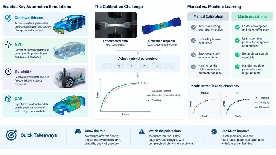
Every crash, rattle, and fatigue crack predicted by CAE software ultimately traces back to a small set of numbers describing how a material behaves. In automotive engineering, material parameter calibration is the process of fitting constitutive model parameters so that a simulation reproduces physical test data — a tensile coupon, a drop tower, a shaker table, a four-post rig — within an acceptable error band. The parameters themselves are rarely measured directly. They are inferred, and that inference is where most of the engineering effort lives.
This chapter establishes the role of calibration across four CAE domains, examines why manual calibration collapses under production workloads, and frames the motivation for machine learning approaches developed throughout the rest of the course.
Where Calibrated Parameters Enter the CAE Workflow
Consider a typical body-in-white (BIW) program. The CAE chain begins with material cards: *MAT_PLASTIC_KINEMATIC, *MAT_024, *MAT_187 (SAMP-1), GISSMO damage tables, or frequency-dependent viscoelastic definitions. Each card contains parameters that must be tuned against experimental data before the model is trustworthy. The same steel grade may require different calibration sets depending on strain rate regime, temperature, and forming history.
The four domains place distinct demands on those parameters:
- Crashworthiness: Large plastic strain, strain rates from 0.001 to 1000 s⁻¹, failure and fracture. Parameters include yield stress scaling, hardening curve coefficients (Swift, Voce, or combined), strain-rate sensitivity (Cowper–Symonds
Dandp, or Johnson–CookC), and damage initiation/evolution terms. A 5% error in flow stress at 200 s⁻¹ can shift intrusion predictions by tens of millimeters. - NVH: Small-strain, frequency-domain behavior. Parameters include complex modulus, loss factor, damping ratio, and frequency-dependent stiffness for elastomers and adhesives. Calibration targets come from DMA sweeps and modal tests rather than quasi-static tension.
- Durability: Cyclic plasticity and fatigue. Parameters include kinematic hardening (Chaboche
C_i,γ_i), isotropic hardening saturation, and strain-life coefficients (Coffin–Mansonε_f',c; Basquinσ_f',b). Load histories are long, so small parameter biases accumulate over millions of cycles. - General CAE (stiffness, modal, forming): Elastic constants, orthotropic directions for composites, and thermal expansion. These are often the easiest to calibrate but still require consistency checks across domains.
The critical point is that these domains are coupled through shared material definitions. A hardening curve tuned for crash may degrade NVH correlation if the same card is reused. Calibration is therefore not a single-task problem but a multi-objective one.
The Manual Calibration Loop and Its Failure Modes
A conventional manual workflow looks like this: an engineer runs a coupon simulation in LS-DYNA or Abaqus, compares the force–displacement curve to the test, adjusts parameters by hand or with a spreadsheet, and repeats. With three to five parameters this converges in a day. With fifteen parameters and multiple loading conditions, it becomes a week-long exercise in trial and error.
Three failure modes dominate:
- Non-uniqueness: Different parameter combinations produce nearly identical coupon curves but diverge under structural loading. Manual tuning cannot explore this space systematically.
- Scalability: A modern vehicle program may involve 40+ material grades, each with multiple strain-rate and temperature conditions. Manual calibration does not scale to hundreds of parameter sets.
- Reproducibility: When calibration is driven by engineer intuition, the result depends on who ran it. Recalibrating after a test update often produces a different parameter set with no clear justification.
Why Machine Learning Changes the Economics
Machine learning reframes calibration as a surrogate-assisted inverse problem. Instead of guessing parameters and running forward simulations, we train a model that maps test observables (curves, modal frequencies, hysteresis loops) back to parameters, or we train a fast surrogate of the simulator and optimize against it. The surrogate can evaluate thousands of candidates per second, enabling global search, uncertainty quantification, and multi-objective trade-offs.
The practical benefits are concrete: calibration time drops from days to hours, parameter sets become reproducible because the optimizer is deterministic given the same data, and sensitivity information falls out of the model for free. The remainder of this course builds the specific techniques — design of experiments, Gaussian process surrogates, neural network inverse models, and Bayesian optimization — on top of the domain context established here.
What a Calibration Task Actually Looks Like
To make this concrete, consider a dual-phase steel DP780 coupon tested at four strain rates: 0.001, 0.1, 10, and 500 s⁻¹. The constitutive model is *MAT_024 with a Voce hardening law and Cowper–Symonds rate scaling. The parameter vector is θ = [σ_y, Q, b, D, p], where σ_y is initial yield, Q and b control saturation, and D, p govern rate sensitivity.
A manual engineer would adjust these five values across four curves — twenty degrees of freedom in practice. A surrogate-based approach instead samples the parameter space with a Latin hypercube of, say, 200 points, runs the coupon simulation at each, trains a Gaussian process mapping θ → curve error, and runs Bayesian optimization for 50 iterations. The result is a parameter set that minimizes weighted RMSE across all four rates simultaneously.
Verification is straightforward: plot simulated versus experimental engineering stress–strain curves at each rate. A well-calibrated set should keep the maximum flow-stress error below 3% and the energy-absorption error below 5% across the range. If the 500 s⁻¹ curve diverges while the quasi-static curves match, the rate-sensitivity parameters D and p are under-constrained — a classic symptom that manual tuning often masks by overfitting one curve at the expense of others.
The Road Ahead
The rest of this course moves from this domain foundation into the mechanics of surrogate modeling, experimental design, inverse neural networks, and multi-objective calibration. Each technique is presented in the context of the four CAE domains introduced here, with worked examples using realistic automotive material data. The goal is not to replace engineering judgment but to give it a faster, more systematic, and more reproducible toolset.