1. Automotive crash CAE landscape
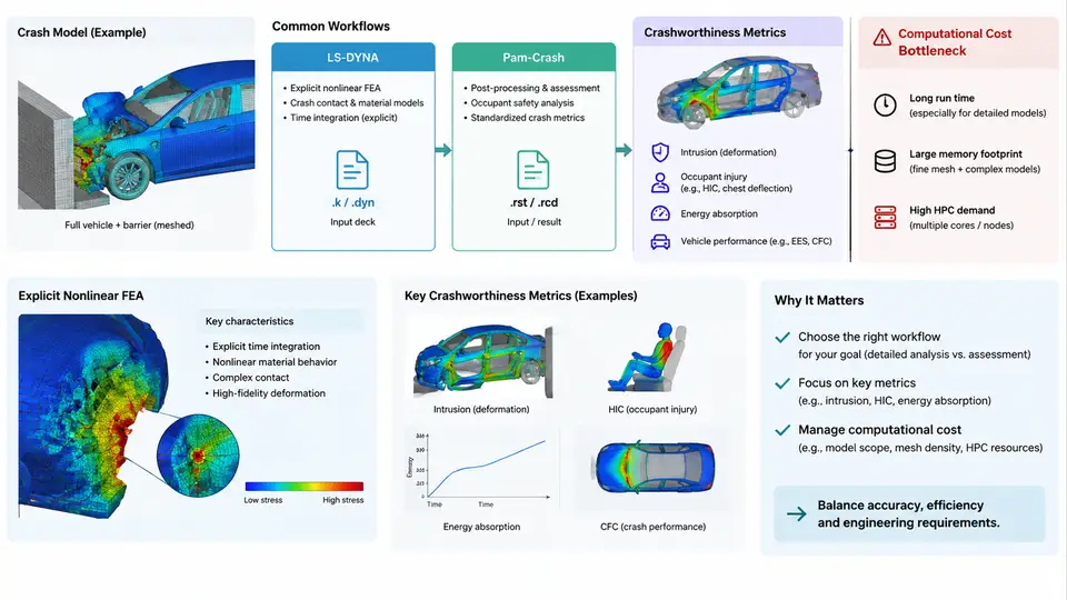
Crashworthiness engineering is one of the most computationally demanding disciplines in automotive CAE. Before any surrogate model can be trained, validated, or deployed, an engineer must understand the simulation stack it is meant to accelerate. This chapter maps that stack: the physics of explicit nonlinear finite element analysis (FEA), the two dominant solvers in production use (LS-DYNA and Pam-Crash), the metrics that define a "good" crash result, and the computational cost structure that motivates surrogate modeling in the first place.
Why Crash Simulation Is Explicit and Nonlinear
A frontal offset impact at 64 km/h (40% overlap, per Euro NCAP / IIHS-style protocols) unfolds in roughly 80–120 ms. Within that window, sheet-metal components fold, spot welds rupture, airbags deploy, and occupants load belts and pretensioners. Three physical characteristics force the choice of an explicit time-integration scheme:
- Large deformation and contact: Shell elements undergo buckling and self-contact; the stiffness matrix changes continuously, so implicit Newton iterations struggle to converge.
- Short, high-frequency event: The characteristic time is milliseconds, so the central-difference method's small stable time step is acceptable.
- Highly nonlinear material response: Strain-rate-dependent steels (e.g., DP590, HSLA340) and failure criteria (Johnson–Cook, GISSMO) require incremental integration.
The explicit central-difference update solves the equation of motion M·a = F_ext − F_int without assembling or factorizing a global stiffness matrix. The stable time step is governed by the Courant condition:
Δt_crit = L_e / c,   c = sqrt(E / ρ)

L_e  = characteristic element length (mm)
E    = Young's modulus (MPa)
ρ    = density (t/mm³)
c    = sound speed in the material (mm/ms)
For a typical steel shell element with L_e = 5 mm, E = 210000 MPa, and ρ = 7.85e-9 t/mm³, the sound speed is about 5170 mm/ms, giving Δt_crit ≈ 0.97 µs. A 100 ms event therefore requires on the order of 10⁵ time steps — and each step touches every element in a model that may contain 5–15 million elements.
LS-DYNA and Pam-Crash Workflows
LS-DYNA (Ansys) and Pam-Crash (ESI) dominate automotive crash simulation. Both use explicit time integration and share a similar preprocessing–solve–postprocessing pipeline, but differ in solver internals, contact algorithms, and keyword conventions.
| Aspect | LS-DYNA | Pam-Crash |
|---|---|---|
| Input format | Keyword deck (*CONTROL, *MAT, *PART) | Pam-Crash input deck (/MAT, /PART, /RUN) |
| Contact | *CONTACT_AUTOMATIC_SINGLE_SURFACE | Self-impact / sliding interfaces |
| Typical element count | 5–15 M shells + solids | 5–15 M shells + solids |
| Wall-clock per run | 8–48 h on 64–256 cores | 8–48 h on 64–256 cores |
| Common preprocessor | ANSA, HyperMesh, LS-PrePost | ANSA, HyperMesh, Visual-Crash |
A production workflow typically proceeds as follows. The CAD body-in-white is meshed with shell elements (target 5–8 mm), spot welds are represented as rigid or beam elements, and materials are assigned from coupon-test-derived curves. Boundary conditions include a rigid barrier, initial velocity, and gravity. The solver writes a d3plot (LS-DYNA) or DSY (Pam-Crash) binary result file at a fixed output interval, from which postprocessors extract deformation, acceleration, and force histories.
Crashworthiness Metrics
Engineers judge a crash result against a small set of scalar and time-history metrics. These are exactly the quantities a surrogate model must predict.
- Intrusion: Maximum displacement of the firewall or dash panel into the occupant compartment (e.g., < 150 mm target).
- B-pillar / rocker acceleration: Peak deceleration at the seat-track attachment, often filtered per SAE J211 (CFC 60).
- Energy absorption: Internal energy of the front rail and crash box, integrated over the event.
- HIC (Head Injury Criterion): Derived from occupant head acceleration; a regulatory and consumer-test threshold.
- Section force: Force transmitted through the front rail at a defined cross-section, used to tune the crash pulse.
Each metric is a nonlinear function of dozens of design variables — gauge thickness, material grade, bead geometry, weld spacing, and trigger initiators. A single design-of-experiments (DOE) study may require hundreds of runs.
The Computational Cost Bottleneck
The cost of a single crash run is the product of model size, time-step count, and contact-search overhead. A representative 10-million-element model on 128 cores consumes roughly 20,000 core-hours. A 200-run DOE therefore costs about 4 million core-hours — weeks of wall-clock time on a shared cluster, and a queue that blocks design iteration.
This bottleneck is the central motivation for surrogate modeling. If a machine-learning model can predict intrusion, peak acceleration, and energy absorption from design variables in milliseconds instead of hours, engineers can explore the design space interactively, run optimization loops, and reserve full FEA for final validation.
What This Means for Surrogate Modeling
The landscape described above defines the surrogate modeling problem precisely. The inputs are design variables (thickness, material grade, geometry parameters); the outputs are crashworthiness metrics (intrusion, peak acceleration, energy absorption, HIC). The training data comes from explicit FEA runs, each costing hours to days. The surrogate must be accurate enough to guide design decisions while being fast enough to replace the solver in an optimization loop.
In the chapters that follow, we will build surrogates for exactly these quantities — starting with data generation strategies that maximize information per expensive FEA run, then moving to model architectures, validation protocols, and deployment in production crash CAE workflows.