1. Crashworthiness simulation landscape
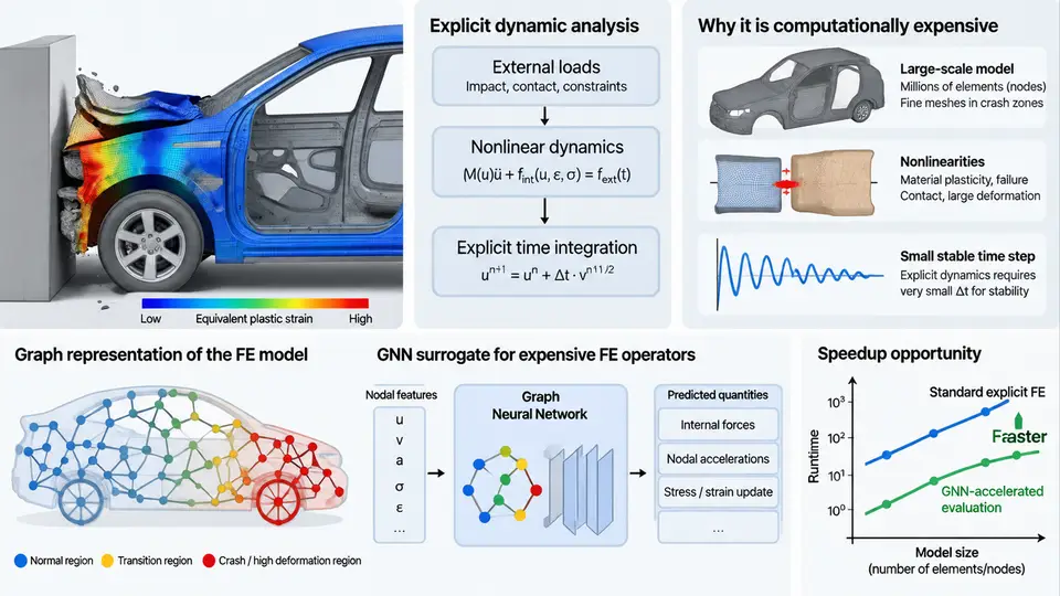
Crashworthiness engineering asks a deceptively simple question: when a vehicle structure strikes a barrier, how does it deform, and does the occupant compartment survive intact? Answering that question numerically is the job of explicit finite element analysis (FEA), and the way that analysis is formulated determines both its physical fidelity and its computational cost. This chapter establishes the simulation landscape that the rest of the course builds on: how explicit dynamics works, why crash models are so expensive, and which specific bottlenecks graph neural networks (GNNs) are positioned to relieve.
Why Crash Simulation Uses Explicit Time Integration
Crash events are short, violent, and highly nonlinear. A frontal impact develops over roughly 80–150 ms, involves strain rates of 10²–10⁴ s⁻¹, large plastic deformation, self-contact, and material failure. The governing semi-discrete equation of motion is:
M · a(t) + C · v(t) + F_int(u(t)) = F_ext(t)where M is the mass matrix, C the damping matrix, F_int the internal (element) force vector, and F_ext the applied load. In an implicit solver, equilibrium is enforced at time t+Δt by solving a nonlinear system with the tangent stiffness matrix K_T at every iteration. That approach is robust for static or slow problems, but during crash it suffers from repeated factorizations of a large, ill-conditioned, contact-dependent K_T, and convergence frequently fails when elements invert or contacts switch.
Explicit integration sidesteps the linear solve entirely. With a lumped (diagonal) mass matrix, accelerations follow directly from force summation:
a_n = M⁻¹ · (F_ext,n − F_int,n − C · v_n)
v_{n+1/2} = v_{n−1/2} + a_n · Δt
u_{n+1}   = u_n + v_{n+1/2} · Δt
No matrix inversion, no Newton iteration, no convergence failure. The price is conditional stability: the central-difference scheme is stable only if the time step satisfies the Courant–Friedrichs–Lewy (CFL) condition, approximated for a linear element as Δt ≤ 2/ω_max, or more practically Δt = L_e / c, where L_e is the smallest element characteristic length and c is the dilatational wave speed c = √(E/ρ). For automotive steel with E ≈ 210 GPa and ρ ≈ 7.85 × 10⁻⁹ t/mm³, c ≈ 5.2 mm/µs. A 5 mm shell element therefore yields Δt ≈ 1 µs — meaning a 100 ms event requires on the order of 100,000 time steps.
The Anatomy of a Production Crash Model
A full-vehicle frontal impact model typically contains 5–15 million elements, dominated by shell elements for the body-in-white, with solid elements for castings and battery enclosures, plus spot welds, adhesives, and rigid barriers. Each time step evaluates element forces, hourglass control, contact search and penalty forces, and material constitutive updates. Contact is often the single largest cost: a 10-million-element model may generate hundreds of thousands of active contact pairs, and the search must be repeated as surfaces move.
The practical consequences are well known to every CAE engineer:
- Turnaround time. A single 100 ms frontal impact on 32–64 CPU cores runs for 8–24 hours. A design-of-experiments (DOE) study with 200 variants consumes weeks of cluster time.
- Time-step collapse. One distorted element with
L_e = 0.4 mmforcesΔtdown by an order of magnitude, and the entire model pays for it. Mass scaling is the standard remedy, but it alters inertia and must be audited. - Contact churn. Penalty stiffness, friction, and self-contact switching introduce high-frequency noise that can dominate the response if not filtered.
- Non-smooth nonlinearity. Element deletion, rupture criteria, and spot-weld failure make the force–displacement response piecewise and non-differentiable — hostile territory for gradient-based optimization.
Where the Cost Actually Lives
It is tempting to treat the solver as a monolith, but the bottlenecks are separable, and each maps to a different class of surrogate model. The diagram below decomposes a crash solve into its dominant cost centers and shows which ones GNN surrogates target.
What Makes This Problem a Natural Fit for GNNs
An FE mesh is already a graph: nodes are vertices, elements define edges, and nodal connectivity is sparse and local. GNN message passing mirrors the stencil operation of an FE solver — each node aggregates information from its neighbors, exactly as an element computes forces from its nodes. This structural correspondence is why GNNs outperform dense surrogates (MLPs, CNNs on voxelized geometry) on crash problems: they respect the irregular topology, generalize across mesh resolutions, and scale with local connectivity rather than global grid size.
Three properties of crash simulation make the mapping especially productive:
- Locality. Explicit dynamics is a local operator. A node's next state depends only on its immediate neighbors and its own history. GNN receptive fields align naturally with the CFL-limited domain of dependence.
- Permutation and resolution invariance. The same physical structure meshed at 3 mm or 5 mm should produce the same response. Graph-based models can be trained to respect this, whereas grid-based models cannot.
- Parametric generalization. Design variants (gauge thickness, material grade, bead layout) can be encoded as node or edge features, letting one trained model cover a family of designs rather than a single configuration.
What GNNs Cannot Replace
A realistic course must state the limits clearly. GNN surrogates are not a drop-in replacement for the explicit solver in certification. They struggle with:
- Long-horizon rollout. Autoregressive prediction accumulates error; a model accurate for 5 ms may drift badly by 80 ms. Stability of the learned propagator is an open research problem.
- Unseen failure modes. Element deletion, rupture, and weld fracture are discontinuous events poorly represented in smooth regression.
- Certification and traceability. Regulatory crash assessment requires a verifiable physical solver. GNNs currently serve as screening, optimization, and design-space exploration tools, not as the final authority.
The Bottleneck Map You Will Reuse
Keep the following decomposition in mind throughout the course, because each subsequent chapter targets one row:
| Bottleneck | Physical origin | GNN approach | Typical target gain |
|---|---|---|---|
| Time-step count | CFL limit from smallest element | Learned propagator with larger effective Δt | 10–100× fewer steps |
| Contact evaluation | Penalty search over active pairs | Graph contact surrogate | 2–5× on contact-dominated models |
| Design iteration | Full solve per variant | Parametric response GNN | Hours → seconds |
| Optimization gradients | Non-smooth, non-differentiable response | Differentiable GNN surrogate | Enables gradient-based design |
The remainder of this course moves from this landscape into the concrete machinery: how to build the mesh graph, how to formulate the message-passing operator for dynamic problems, how to generate and curate training data from explicit solves, how to enforce physical constraints such as momentum conservation, and how to validate a surrogate against the solver it is meant to accelerate. The starting point is always the same question: which bottleneck are you attacking, and what does the physics of that bottleneck demand from the model?