1. Digital twin fundamentals for automotive
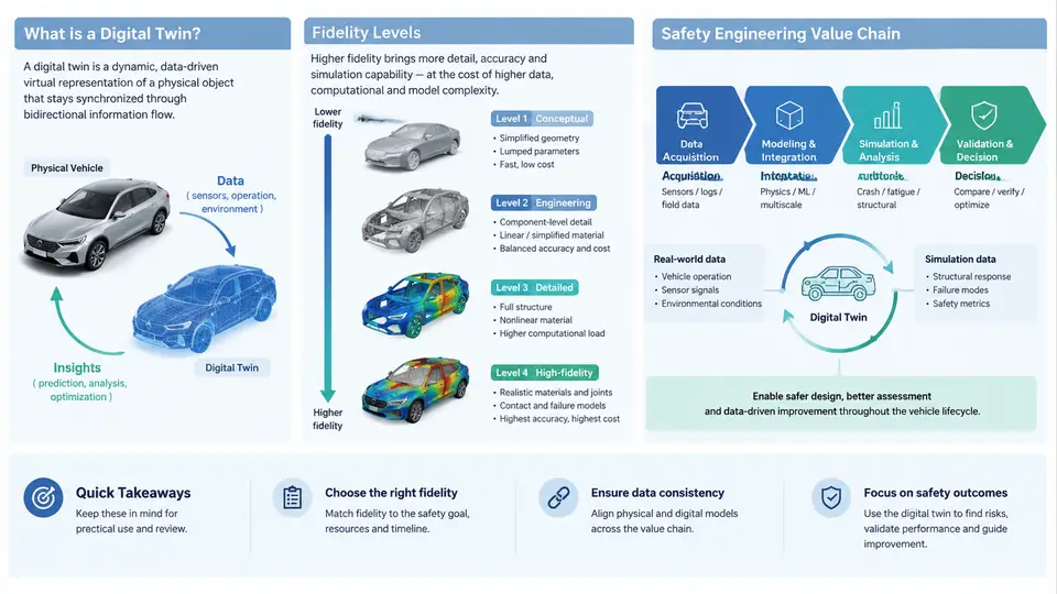
A digital twin is not simply a 3D model of a vehicle body. In automotive structural safety engineering, a digital twin is a living, data-connected virtual representation of a physical structure — a body-in-white, a battery enclosure, a full vehicle — that stays synchronized with its real counterpart across the entire lifecycle. The defining characteristic is bidirectional information flow: sensor data, test results, and field incidents update the model, while the model informs design decisions, inspection intervals, and safety margins.
This distinction matters because structural safety is a lifecycle problem. A crash simulation run once during design verification is a model. The same simulation, continuously recalibrated with fleet crash data, manufacturing variation measurements, and in-service strain monitoring, becomes a digital twin. The difference is not the solver or the mesh density — it is the persistent, closed-loop connection to physical reality.
Definitions and Core Architecture
In the automotive safety context, we can define a digital twin along three axes:
- Physical entity: the actual structure under consideration — a specific vehicle identification number (VIN), a production batch, or a design variant.
- Virtual entity: the computational model — finite element (FE) model, reduced-order model (ROM), or hybrid surrogate — that predicts structural response.
- Connection layer: the data pipeline that transfers measurements, updates model parameters, and returns predictions or decisions.
The connection layer is where most engineering effort is spent. It includes sensor networks (strain gauges, accelerometers, crash test dummies, event data recorders), data assimilation algorithms (Kalman filters, Bayesian updating, machine learning surrogates), and decision interfaces (inspection scheduling, recall triggers, design change recommendations).
Fidelity Levels: Choosing the Right Resolution
Fidelity in structural safety digital twins is not a single number. It spans multiple dimensions: geometric detail, material model complexity, mesh resolution, time integration scheme, and the frequency of data synchronization. The following table summarizes four commonly used fidelity tiers in automotive structural safety practice.
| Level | Typical Model | Use Case | Update Frequency | Computational Cost |
|---|---|---|---|---|
| L0 — Conceptual | 1D lumped-parameter or beam models | Early architecture trade studies, load path screening | Static | Seconds |
| L1 — System-level | Coarse FE (10–30 mm mesh), simplified material laws | Full-vehicle crashworthiness, occupant restraint optimization | Per design iteration | Hours |
| L2 — Component-level | Fine FE (2–5 mm mesh), calibrated plasticity and failure models | B-pillar, rocker, battery enclosure detailed analysis | Per test campaign | Days |
| L3 — Local/hotspot | Sub-modeling, crystal plasticity, weld/spot joint detail | Fatigue crack initiation, weld failure, corrosion effects | Continuous (with monitoring data) | Hours per update |
The choice of fidelity level is a trade-off between predictive accuracy and the ability to update the model within the decision window. For a fleet-level recall decision, an L1 model updated weekly may be sufficient. For a single vehicle approaching a critical inspection, an L3 hotspot model updated with real-time strain data is more appropriate.
The Safety Engineering Value Chain
Digital twins create value at every stage of the automotive structural safety value chain. Understanding this chain helps engineers position their twin correctly and avoid over-engineering.
Design and virtual verification. During concept and detailed design, the twin is primarily a simulation model. Value comes from reducing physical prototypes, exploring design variants, and identifying critical load paths. The twin is not yet connected to a physical asset, but it establishes the baseline model that will later be calibrated.
Physical testing and model calibration. Crash tests, sled tests, and component tests provide the ground truth. The digital twin is updated by adjusting material parameters, boundary conditions, and joint stiffnesses to match measured responses. This is the first true synchronization event. A common pitfall is calibrating only to global metrics (e.g., B-pillar intrusion) while ignoring local strain histories that matter for fatigue and fracture.
Manufacturing and as-built variation. Production introduces variation: sheet metal thickness tolerances, weld nugget size scatter, springback, and residual stresses. A digital twin that ignores these effects will drift from reality. Advanced implementations use in-line measurement data (laser scanning, weld inspection) to update the model for each production batch or even each VIN.
In-service monitoring and prognostics. Once vehicles are on the road, the twin becomes a health-monitoring tool. Strain gauges, accelerometers, and event data recorders feed operational loads into the model. The twin then estimates remaining fatigue life, detects anomalous deformation, and recommends inspection or repair. This is where the digital twin delivers its highest safety value — catching degradation before it becomes a failure.
Incident investigation and feedback. When a crash or structural failure occurs, the digital twin provides a forensic framework. By replaying the event with measured crash pulse and pre-crash load history, engineers can identify whether the failure was due to design, manufacturing, or unexpected service loads. This feedback closes the loop back to design and manufacturing.
Practical Implementation: A Worked Example
Consider a digital twin for a battery enclosure in an electric vehicle. The physical asset is a specific production batch of 500 enclosures. The safety concern is fatigue cracking at weld seams under road-induced vibration and occasional curb impacts.
Step 1 — Baseline model. Build an L2 FE model of the enclosure with shell elements (3 mm mesh) and spot-weld connectors. Material: aluminum 6061-T6 with a calibrated strain-life curve. This model predicts hot-spot locations but not absolute fatigue life.
Step 2 — Sensor placement. Based on the baseline model, place 12 strain rosettes at the top five hot-spot regions. Install accelerometers on the enclosure mounts to capture input loads.
Step 3 — Data assimilation. Every 1,000 km, upload strain histories. Use a rainflow counting algorithm to extract cycles, then apply Miner's rule with the calibrated strain-life curve. Update the model's weld stiffness parameters using a Bayesian calibration against measured strain ranges.
Step 4 — Prognostics. The twin outputs a remaining fatigue life estimate per weld. If any weld's cumulative damage exceeds 0.7, trigger an inspection alert. If it exceeds 0.9, recommend immediate repair.
Step 5 — Verification. After 50,000 km, remove one enclosure from service and perform a physical fatigue test to failure. Compare the twin's predicted life to the actual life. A well-calibrated twin should fall within ±20% for this application.
Common Pitfalls and How to Avoid Them
- Confusing a model with a twin. If the model is not updated with physical data, it is not a twin. Define the update trigger and data pipeline before building the model.
- Over-specifying fidelity. An L3 model that takes three days to update is useless for a decision needed in one hour. Match fidelity to the decision window.
- Ignoring manufacturing variation. A twin calibrated to nominal dimensions will drift. Incorporate as-built measurements whenever available.
- Neglecting uncertainty. Every prediction should carry a confidence interval. A point estimate of remaining life without uncertainty is misleading for safety decisions.
The digital twin is ultimately a decision-support tool. Its value is measured not by the elegance of its mathematics but by the safety decisions it enables: when to inspect, when to repair, when to recall, and when to redesign. The next chapter will examine the specific sensor technologies and data acquisition architectures that make structural safety twins possible.