1. Course overview

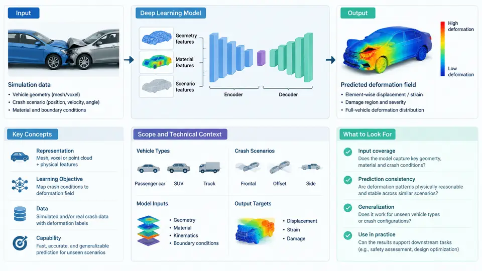
Vehicle crashworthiness engineering has traditionally relied on explicit finite element analysis (FEA), most commonly with LS-DYNA or Radioss, to simulate how a body-in-white (BIW) deforms during an impact event. A single full-vehicle frontal offset simulation at a 1–2 mm mesh resolution can require tens of millions of elements and several hours to several days of wall-clock time on a high-performance computing cluster. When engineers must explore hundreds of design variants — thicknesses, grades, bead patterns, joint layouts — this cost becomes the dominant bottleneck in the development loop. Deep learning enters this picture not as a replacement for FEA, but as a fast surrogate that maps design parameters directly to deformation fields, enabling interactive design space exploration, optimization, and early-stage concept screening.

This course is about building, validating, and deploying such surrogates. It covers the full technical chain: how crash deformation data is represented, how simulation and test data are curated, which neural network architectures are appropriate, how physics constraints are injected, and how predictions are judged against engineering acceptance criteria. By the end, you should be able to take a raw set of crash simulation results and design variables and produce a model that predicts deformation with quantified accuracy and known failure modes.

What "Crash Deformation Prediction" Actually Means

The prediction target is not a single scalar. In practice, deformation is represented in several complementary ways, and the choice of representation drives the entire modeling strategy:

• Scalar responses: intrusion at a specific point (e.g., B-pillar maximum intrusion in mm), occupant compartment volume loss, or peak acceleration at the rocker. These are low-dimensional and easy to regress, but they discard spatial information.
• Field responses: nodal displacement or plastic strain over the full mesh, typically stored as a tensor of shape [N_nodes, 3] for displacement or [N_nodes] for an equivalent plastic strain scalar field. This is the high-value target because it captures buckling patterns, fold initiation, and load path changes.
• Reduced-order representations: modal coordinates, principal component analysis (PCA) coefficients, or autoencoder latent vectors that compress the field into 10–100 dimensions. This is often the practical compromise between fidelity and learnability.

A critical concept is that deformation fields are structured: neighboring nodes move coherently, and the field respects material continuity. A naive multilayer perceptron that treats each node independently will produce physically implausible, noisy outputs. This is why graph neural networks (GNNs), convolutional neural networks (CNNs) on projected images, and point-cloud networks are central to this field.

The Technical Context: Where Deep Learning Fits

It helps to place the surrogate within the existing crash CAE workflow. The diagram below shows the data and model flow from design parameterization through simulation, training, and deployment, with the key interfaces labeled.

Why Deep Learning, and Why Not Classical Surrogates?

Classical response surface methods — polynomial regression, Kriging, radial basis functions — work well when the output is a handful of scalars and the design space is smooth. Crash deformation violates both assumptions. The output is a high-dimensional field, and the input–output relationship contains sharp transitions: a 0.1 mm thickness change can flip a fold initiation site, producing a discontinuous jump in the deformation pattern. Deep networks handle this better for three reasons: they learn hierarchical spatial features, they can be trained on large simulation datasets without hand-crafted basis functions, and they can incorporate physical constraints through the loss function or architecture.

That said, the field has real limitations you must internalize from day one. Deep surrogates extrapolate poorly outside the training distribution. They can produce kinematically inadmissible deformations (self-intersecting elements, non-physical strain concentrations) unless constrained. And they require careful validation against both FEA and physical test data. A model that achieves 2% mean absolute error on a random hold-out set may still fail catastrophically on a design point near the boundary of the training envelope.

Core Concepts You Will Use Throughout

Design parameterization. Every surrogate needs a fixed-length input vector. Typical variables include sheet thickness (0.8–2.0 mm), material grade (DP590, DP780, HSLA340), bead depth, and joint stiffness. Categorical variables such as grade must be encoded, and geometric variables may come from CAD morphing or shape basis coefficients.

Mesh correspondence. For field prediction, all training samples must share a consistent node ordering. If meshes differ between simulations, you must either remesh to a common topology or use a correspondence-free representation such as point clouds or signed distance fields.

Dimensionality reduction. PCA on the stacked displacement fields typically retains 95–99% variance with 20–50 modes. The network then predicts these coefficients, and a fixed decoder reconstructs the full field. This is the most common practical architecture and is covered in depth in later chapters.

Physics-informed learning. Loss terms can enforce equilibrium residuals, boundary conditions (fixed nodes at the firewall), or symmetry. A simple and effective constraint is to penalize deviation from known rigid-body motion at the vehicle mounts.

Validation metrics. Do not rely on a single number. Report per-node field RMSE, maximum intrusion error at engineering-critical points, and the correlation of the first few PCA coefficients. A model with low global RMSE but high error at the B-pillar is not acceptable for occupant safety assessment.

Scope Boundaries and What This Course Does Not Cover

This course focuses on supervised learning from simulation data, with validation against physical test data where available. It does not cover real-time sensor-based crash detection, occupant injury prediction (which involves a different biomechanical modeling chain), or full vehicle dynamics. The emphasis is on the deformation field of structural components — front rails, B-pillars, rockers, and floor panels — under frontal and side impact loading. The methods generalize to other impact modes, but the examples and datasets used throughout are drawn from these configurations.

By the end of this chapter, you should understand that crash deformation prediction is a high-dimensional, physics-constrained regression problem where the main challenges are data representation, mesh correspondence, and rigorous validation — not simply choosing a network architecture. The chapters that follow build each of these capabilities in sequence, starting with the data pipeline and ending with deployment in an optimization loop.