1. Airbag deployment response prediction
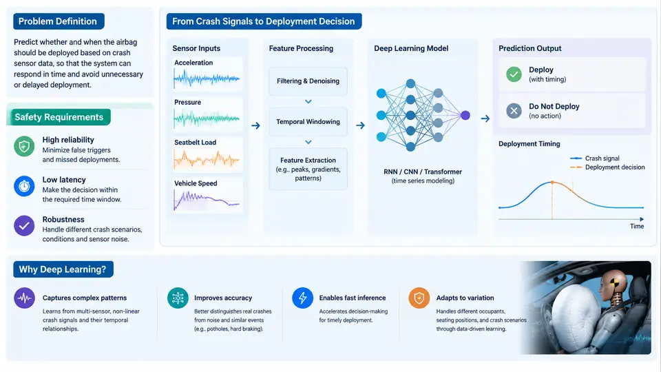
An airbag is a pyrotechnic restraint device that must inflate within tens of milliseconds of a crash signal, then vent and deflate fast enough to absorb the occupant's forward momentum without itself becoming an injury source. The engineering question this course addresses is deceptively simple: given a vehicle, a crash condition, and an occupant state, what will the airbag actually do — and will that behavior satisfy the safety requirements? Predicting that response accurately, early in the design cycle, is the core problem.
1.1 Defining the Prediction Problem
Airbag deployment response is not a single number. It is a time-resolved physical process described by several coupled output channels:
- Bag pressure history
p(t)inside the cushion, driven by the inflator's gas mass flow rate and temperature. - Cushion geometry over time — the expanding membrane surface, its contact area with the occupant, and the vent open area.
- Occupant kinematics — head and chest displacement, velocity, and acceleration, usually summarized as injury criteria such as HIC15, chest deflection, and chest a3ms.
- Deployment timing — the time-to-first-gas (TTFG), the time to full inflation, and the interaction window with the occupant.
Formally, we seek a mapping f from a design and loading vector x to a response vector y(t):
y(t) = f( x ; θ )
x = [ inflator mass flow profile, vent diameter, bag volume,
      fabric permeability, fold pattern, module position,
      impact velocity, impact angle, occupant size, seat position ]
y(t) = [ p(t), bag contact force(t), head a(t), chest deflection(t) ]
The parameters θ represent the physical model — gas thermodynamics, fabric mechanics, and occupant dynamics. In practice, f is evaluated either by physical sled and drop-tower tests or by explicit finite-element simulation (e.g., LS-DYNA or PAM-CRASH with a corpus of validated airbag and dummy models). Both are expensive: a single validated frontal sled test can cost tens of thousands of dollars and consume a vehicle; a single high-fidelity deployment simulation can run for hours on a compute cluster.
1.2 Safety Requirements That Constrain the Response
The prediction is only useful if it is judged against hard regulatory and internal targets. The dominant requirements are:
| Requirement | Typical target | Why it matters |
|---|---|---|
| HIC15 (head injury criterion) | ≤ 700 (FMVSS 208), often ≤ 500 internal | Limits head acceleration exposure |
| Chest deflection | ≤ 63 mm (Hybrid III 50th) | Prevents rib fracture and organ injury |
| Chest a3ms | ≤ 60 g | Limits sustained chest deceleration |
| Out-of-position (OOP) pressure | Bag must not injure a close occupant | Governs inflator output and venting |
| Deployment time | Full inflation in ~30–50 ms | Occupant must be restrained before contact |
These targets are not independent. Increasing inflator mass flow raises pressure and reduces time-to-inflation, but it also raises OOP injury risk and can increase head acceleration. Enlarging the vent lowers peak pressure and softens the cushion, but may delay full inflation and reduce restraint effectiveness. The design space is therefore a tightly coupled, multi-objective trade-off — and every candidate design must be evaluated across a matrix of impact speeds, angles, occupant sizes, and seat positions.
1.3 Why Conventional Methods Reach Their Limits
Two conventional approaches dominate current practice, and both have structural limitations.
Physical testing is the ground truth, but it is destructive, slow, and sparse. A typical development program might run 50–150 sled tests across a matrix of conditions. That sampling density is far too low to resolve the sensitivity of HIC to, say, a 2 mm change in vent diameter or a 5° change in impact angle. Tests also cannot be repeated on the same vehicle, so scatter from build variation and instrumentation is difficult to separate from true design sensitivity.
Finite-element simulation fills the sampling gap but introduces its own cost. A single frontal deployment model with a folded bag, a validated inflator model, and a full dummy can require 106–107 elements and hours of wall-clock time. Running a 200-point design of experiments (DOE) is feasible but expensive; running a 10,000-point sensitivity sweep or a real-time optimization loop is not. Moreover, FE models carry modeling error — fabric permeability, fold initialization, and inflator burn curves are all calibrated approximations — so the simulation is a surrogate for reality, not reality itself.
Classical response surface methods (polynomial regression, kriging, radial basis functions) can accelerate the inner loop, but they struggle when the response is highly nonlinear and time-dependent. A polynomial surrogate cannot represent the sharp pressure spike at inflator onset, the nonlinear venting regime, or the occupant contact transition. Kriging works well for smooth scalar outputs but becomes impractical for full time histories and high-dimensional inputs.
1.4 What Deep Learning Changes
Deep learning offers a different trade: instead of hand-specifying the functional form, we learn it from data. The relevant capabilities are:
- Sequence modeling. Recurrent networks, temporal convolutional networks, and transformers natively consume and emit time series, so they can predict
p(t)and occupant kinematics directly rather than reducing them to scalars. - High-dimensional input handling. A network can ingest dozens of design and loading parameters simultaneously and learn interactions that a polynomial basis would miss.
- Speed after training. Once trained, inference takes milliseconds, enabling real-time design exploration, optimization, and Monte Carlo robustness studies.
- Multi-output and multi-fidelity learning. One model can predict pressure, force, and injury criteria jointly, and can be trained on a mix of cheap FE runs and expensive test data.
The trade-off is data hunger and interpretability. A deep model needs a well-designed training set, careful normalization, and validation against held-out physical tests. It also does not replace physics — it compresses it. The most effective architectures in this domain are physics-informed or hybrid: they embed known constraints (mass conservation, non-negative pressure, monotonic inflation before venting) into the loss function or the network structure.
1.5 What "Good" Prediction Looks Like
A deployable surrogate must satisfy three practical criteria. First, accuracy on held-out conditions: for a test set of crash configurations not seen during training, the predicted peak pressure should fall within roughly 5–10% of the FE reference, and HIC15 within about 10–15%, which is comparable to test-to-test scatter. Second, temporal fidelity: the predicted pressure and force histories must reproduce the shape of the curve — onset slope, peak timing, and venting decay — not just the peak value. Third, physical plausibility: pressure must remain non-negative, inflation must precede venting, and the model must not extrapolate to absurd values outside the training envelope.
1.6 The Road Ahead
This chapter has framed airbag deployment response prediction as a time-series regression problem constrained by a multi-objective safety envelope, and has argued that neither physical testing nor FE simulation alone can provide the sampling density and speed required for modern design exploration. Deep learning surrogates address that gap by learning the input-to-time-history mapping directly, with physics-informed structure to preserve plausibility. The chapters that follow build the full pipeline: data generation and preprocessing, architecture selection for time-series outputs, physics-informed loss design, training and validation strategy, uncertainty quantification, and integration into the design workflow.