1. Course overview
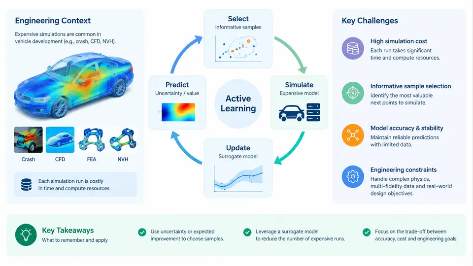
Modern vehicle development depends on simulation to answer questions that physical testing cannot answer cheaply or early enough: How does a battery pack behave during a side-pole impact? Which suspension bushing tuning minimizes road noise at 80 km/h? Does the thermal management strategy keep cell temperatures below the limit during a fast-charge cycle? Each of these questions is answered by a numerical model — typically a finite element (FE) model, a computational fluid dynamics (CFD) model, or a multi-body dynamics (MBD) model — and each simulation run can consume minutes to days of high-performance computing (HPC) time.
This course is about a specific engineering response to that cost: active learning. Instead of running a large design of experiments (DoE) grid and then fitting a surrogate model, active learning builds the surrogate adaptively. It starts with a small initial sample, fits a model that also reports its own uncertainty, and then uses an acquisition function to decide which simulation to run next. The goal is to reach a required prediction accuracy — or to locate an optimum, a failure boundary, or a feasible region — with as few expensive solver calls as possible.
Why Automotive Simulation Is an "Expensive Function"
The term expensive is not rhetorical. Consider three representative cases from vehicle engineering:
- Crashworthiness (LS-DYNA / Pam-Crash): a full-vehicle frontal offset impact model with 8–15 million elements typically runs 6–24 hours on 64–256 cores. A single output of interest (e.g., B-pillar intrusion) is one scalar.
- Battery thermal runaway propagation (CFD): a module-level conjugate heat transfer model with detailed cell kinetics can take 10–40 hours per design point.
- NVH / modal analysis (Nastran / OptiStruct): a trimmed body model with 3–5 million DOF solves in 20–90 minutes, but a full frequency sweep across 200 Hz with 2 Hz resolution multiplies that cost.
When one evaluation costs hours, a 500-point Latin hypercube is not a plan — it is a budget request. Active learning reframes the problem: which 40 or 60 points would tell us the most?
The Core Loop and Its Components
Every active learning workflow for simulation has the same skeleton, even though the implementations differ widely:
- Design space definition: bounded input variables (sheet thickness, material parameters, cell spacing, controller gains) with physically meaningful ranges.
- Initial design: a small space-filling sample (often 5–15 points via Latin hypercube or Sobol sequence) to seed the model.
- Surrogate model: a regressor that provides both a prediction and a variance — Gaussian process (Kriging), Bayesian neural network, or ensemble of trees.
- Acquisition function: a scalar score over the design space balancing exploitation (low predicted value) and exploration (high uncertainty). Common choices: Expected Improvement (EI), Lower Confidence Bound (LCB), or probability of feasibility.
- Stopping criterion: maximum EI below a threshold, prediction variance below a tolerance, or a fixed evaluation budget.
The critical difference from classical DoE is step 4: the next simulation point is chosen after seeing the previous results, and the choice is driven by the model's own uncertainty estimate.
Key Challenges in the Automotive Context
Active learning is well established in machine learning benchmarks, but automotive simulation imposes constraints that change how the loop must be built.
1. Heterogeneous, noisy, and sometimes failed evaluations. A crash simulation may terminate early due to element distortion, returning no useful output. A CFD run may converge to a different steady state depending on initial conditions. The surrogate must handle missing data and non-deterministic outputs. In practice, this means either filtering failed points, modeling the failure probability separately, or using a classifier to define a feasible region before optimizing.
2. Mixed variable types. Automotive design variables are rarely all continuous. Sheet thickness is continuous; material grade is categorical (DP600, DP780, HSLA340); the presence of a reinforcement patch is binary. Standard Gaussian processes assume continuous inputs, so categorical variables require either separate models per category, or a modified kernel (e.g., Gower distance or one-hot encoding with ARD).
3. Multi-objective and constrained problems. A crashworthiness study rarely optimizes a single number. It typically trades off mass, intrusion, and peak acceleration, subject to constraints such as "intrusion ≤ 150 mm" and "HIC ≤ 700." Active learning for multi-objective problems uses acquisition functions like Expected Hypervolume Improvement (EHVI), while constrained problems use probability of feasibility as a multiplier.
4. High-dimensional design spaces. A full vehicle model may have 30–80 design variables. Gaussian processes scale poorly beyond ~20 dimensions without dimension reduction. Common remedies include active subspaces, partial least squares, or switching to Bayesian neural networks that handle higher dimensions more gracefully.
5. Integration with existing CAE workflows. The active learning loop must call the solver, parse its output, and feed results back — often across different file formats (LS-DYNA binout, Nastran .f06, CFD .csv). This is an engineering integration problem as much as a mathematical one.
Engineering Context: Where This Fits in the Development Process
Active learning is not a replacement for simulation; it is a layer on top of it. In a typical vehicle program, it appears in three places:
| Phase | Typical Use | Evaluation Budget |
|---|---|---|
| Concept / architecture | Explore material and topology trade-offs; identify feasible design region | 30–80 solver runs |
| Detailed design | Optimize thickness distribution, joint stiffness, or thermal management | 50–150 solver runs |
| Validation / robustness | Quantify uncertainty from material scatter and manufacturing tolerances | 100–300 solver runs |
The value proposition is straightforward: if a conventional DoE would need 500 runs and active learning reaches the same accuracy in 60, the saving is not just compute cost — it is calendar time. In an industry where a one-week delay in a crash model can shift a milestone, that difference matters.
What This Course Covers
Over the following chapters, we will move from the mathematical foundations of Gaussian process surrogates and acquisition functions, through practical implementation details (sampling strategies, kernel selection, handling categorical variables), to full case studies in crashworthiness, NVH, and battery thermal management. Each chapter includes concrete parameter choices, code or configuration examples, and criteria for judging whether the surrogate is trustworthy enough to replace a solver run.
The first practical question is always the same: what does "expensive" mean for your model, and how many runs can you actually afford? That number — the evaluation budget — shapes every subsequent decision in the active learning loop.