1. Crash simulation campaign landscape
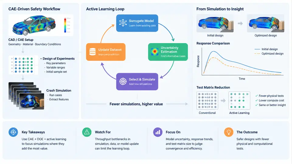
Vehicle safety development is a CAE-driven process. Before a single prototype is built, the crashworthiness, restraint-system, and occupant-protection performance of a vehicle body is explored almost entirely in the virtual domain. A crash simulation campaign is the organized set of CAE runs that a safety team executes to answer a defined engineering question: does this body structure, restraint calibration, or material mix meet the target, and how sensitive is that answer to the design variables we are allowed to change?
Understanding the campaign landscape matters because active learning does not replace CAE — it reorganizes which simulations get run, in what order, and how many. To use it well, you first need a clear picture of the workflow it sits inside, the design space it explores, and the bottlenecks that make naive sampling expensive.
The CAE-driven safety workflow
A typical frontal-offset or side-impact program moves through a recognizable chain. The body-in-white (BIW) and closure geometry arrive from CAD. The team builds a full-vehicle FE model — shell elements for the body, solid and shell meshes for the powertrain and suspension, a deformable barrier, and a validated dummy model such as a THOR or WorldSID occupant. Load cases are defined by regulation or internal targets: FMVSS 208, Euro NCAP MPDB, IIHS small overlap, and so on. Each run produces a time history of accelerations, intrusions, and injury criteria — HIC, chest deflection, femur load, Nij.
The engineering question is rarely "run one crash." It is "find a design that satisfies all criteria across all load cases, with margin, at acceptable mass and cost." That is a multi-objective, multi-constraint optimization problem, and it is where the campaign becomes large.
Design of experiments and the test matrix
Classical Design of Experiments (DoE) is the traditional way to structure the campaign. A full factorial over, say, 8 variables at 3 levels each would require 38 = 6,561 runs — computationally impossible for a full-vehicle model that takes hours per run. Engineers therefore use space-filling or screening designs:
- Latin Hypercube Sampling (LHS) — spreads points evenly across each variable's range; good for building response surfaces.
- Fractional factorial / Plackett-Burman — screens many variables cheaply to find the few that matter.
- Central Composite / Box-Behnken — efficient for fitting quadratic surrogate models.
Each design point is a vector of variable settings: gauge thicknesses, material grades, bead depths, spot-weld pitch, and restraint parameters such as airbag vent size or pretensioner firing time. The test matrix is the table of these points crossed with load cases. Its size is the product of design points and load cases, and it is the primary cost driver of the campaign.
Throughput bottlenecks
Three bottlenecks dominate a crash campaign, and they are not all computational:
| Bottleneck | Typical symptom | Root cause |
|---|---|---|
| Solve time | Runs queue for days | Explicit solver time step limited by smallest element; contact complexity |
| Model build & QA | Failed runs, negative volumes | Manual meshing, inconsistent includes, unit errors |
| Result extraction | Engineers drown in d3plot files | No automated criteria extraction; manual post-processing |
The third bottleneck is often underestimated. A campaign that produces 300 runs but requires an engineer to open each one and read HIC from a plot is not a 300-run campaign — it is a 300-hour post-processing campaign. Automation of criteria extraction is a prerequisite for any active-learning loop, because the loop must read objective values programmatically to decide where to sample next.
Where active learning changes the economics
Active learning reframes the campaign as a sequential decision problem. Instead of committing to a fixed DoE up front, the loop does this:
- Run a small initial design (e.g., 12–20 LHS points).
- Fit a surrogate model — Gaussian Process, Kriging, or a neural network — to the observed responses.
- Use an acquisition function (Expected Improvement, Probability of Feasibility, or a multi-objective variant) to score candidate points.
- Select the most informative or most promising point, run the expensive simulation, and update the model.
- Repeat until the design target is met or the budget is exhausted.
The key insight is that active learning spends simulation budget where it reduces uncertainty or improves the objective, rather than filling a pre-defined grid. In practice, teams report reaching comparable design quality with 30–60% fewer full-vehicle runs — but the exact saving depends on how smooth the response surface is and how many constraints are active.
What the campaign must deliver
Regardless of method, a crash simulation campaign must produce four things: a feasible design that meets all injury and intrusion targets, a sensitivity ranking of which variables drive each response, a margin assessment showing how close the design sits to each constraint, and a traceable record linking every run to its input vector and extracted criteria. Active learning changes how efficiently these are obtained, but not what they are.
Reading the diagram
The left column shows the classical campaign: the matrix is fixed before any result is known, so every run is paid for regardless of whether it adds information. The right column shows the active-learning campaign: the matrix grows one point at a time, and each new point is chosen because the current surrogate is uncertain there or because the acquisition function expects improvement. The dashed orange arrow is the feedback loop — the mechanism that makes the campaign adaptive rather than pre-committed.
Two practical consequences follow. First, the active-learning loop requires a fast, reliable surrogate refit and automated criteria extraction; if either is manual, the loop stalls. Second, the loop needs a stopping criterion — typically a convergence threshold on the best feasible objective, a maximum run budget, or a stability check on the surrogate's predicted improvement. Without one, the campaign never terminates.
With this landscape in view — the CAE workflow, the DoE matrix, the three bottlenecks, and the adaptive loop — the next chapters build the machinery: surrogate models, acquisition functions, constraint handling, and the orchestration that ties them to a real solver queue.