1. Transient shock response simulation for
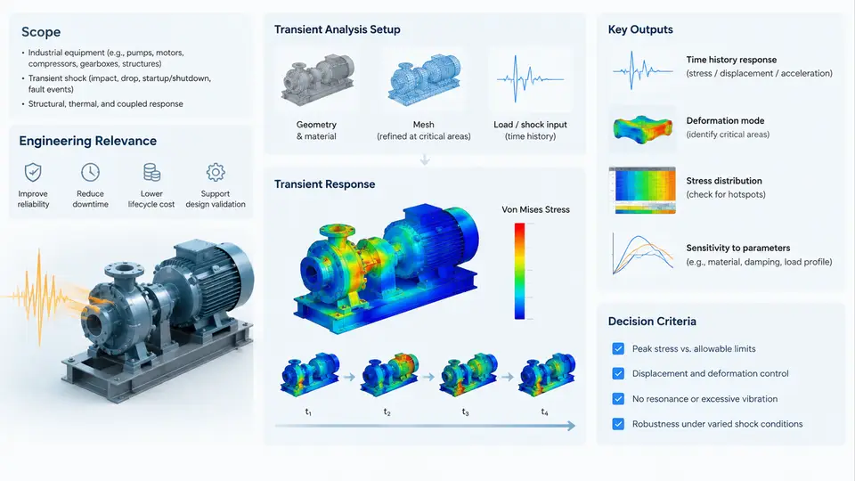
Industrial equipment rarely fails because of steady loads. A pump skid that has run for a decade under constant pressure can crack its mounting bracket the first time it is dropped from a loading dock, struck by a forklift, or subjected to a seismic event. Transient shock response simulation exists to answer a deceptively simple question: when a short, violent, broadband excitation hits a structure, how does that structure actually respond — and will it survive?
This course develops the full engineering workflow for answering that question in a simulation-driven design context. Over 30 chapters we move from the physics of shock excitation, through finite element model preparation, solver configuration, and post-processing, to design decisions and verification. This opening chapter defines the scope of the discipline, explains why it matters commercially and technically, and establishes the modelling philosophy that the rest of the course builds on.
What "Transient Shock" Actually Means
A shock is a transient excitation of relatively short duration that produces a significant response in a structure. The key word is transient: the excitation is not periodic, and the response is dominated by the structure's own dynamics rather than by the forcing function alone. Three physical characteristics distinguish shock from vibration:
- Short duration relative to natural periods. A shock pulse may last 2–20 ms, while the equipment's first bending mode might sit at 40 Hz (25 ms period). The pulse and the structure interact, and the response depends strongly on the ratio of pulse duration to natural period.
- Broadband frequency content. A half-sine pulse of 5 ms duration excites energy across roughly 0–400 Hz. Unlike a sine sweep, it energizes many modes simultaneously.
- High peak acceleration, low velocity change. A 50 g, 5 ms half-sine pulse imparts a velocity change of only about 1.56 m/s, yet the inertial forces during the pulse are large enough to yield brackets and shear fasteners.
Typical sources in industrial equipment include drop and handling events, rail and road transport shock, seismic ground motion, pressure surges and water hammer in piping, blade-loss or rotor-jam events in rotating machinery, and blast or impact loading in process plants.
Why Simulation Instead of Testing Alone
Shock testing on a shaker table or drop tower remains the definitive verification method, and standards such as MIL-STD-810 Method 516, IEC 60068-2-27, and ASTM D3332 define how it is done. So why simulate?
Testing tells you whether a specific article survived a specific pulse. Simulation tells you why, where, and how much margin remains. A drop test produces a pass/fail result and a handful of accelerometer traces. A transient FE analysis produces the full displacement, stress, and reaction-force field at every time step, letting an engineer see that the failure initiates at a weld toe on the third bracket, driven by the second bending mode, at t = 6.2 ms. That diagnostic resolution is what makes design iteration possible before hardware exists.
Simulation also covers cases that are impractical to test: a 12-ton compressor skid that no available shaker can drive, a seismic event with a site-specific response spectrum, or a hundred parametric variants of a bracket thickness. In a simulation-driven design process, transient shock analysis becomes a design tool used at concept and detail stages, with physical testing reserved for final qualification.
The Simulation-Driven Design Context
Transient shock simulation does not sit in isolation. It is one analysis type within a broader CAE workflow, and its inputs and outputs connect to other disciplines. The diagram below shows how a shock analysis is positioned: excitation definition and structural model feed the solver, the solver produces time-history results, and those results feed both design decisions and verification evidence.
Scope of the Course
The course is organized around the workflow shown above, but the emphasis is on engineering judgement rather than software button-pushing. The chapters cover:
- Physics and excitation modelling — pulse shapes (half-sine, terminal-peak sawtooth, trapezoidal), Shock Response Spectrum (SRS) construction, and how to convert a test specification into a solver-ready input.
- Model preparation — mesh density for wave propagation, mass scaling in explicit analyses, contact definition for bolted and welded joints, and boundary condition selection for base-excited equipment.
- Solver configuration — implicit versus explicit time integration, time step selection, Rayleigh damping calibration, and energy balance checks.
- Post-processing and interpretation — reading time-history plots, identifying peak stress locations, computing margins of safety, and distinguishing numerical artefacts from real response.
- Design application — isolator selection, bracket optimization, and the correlation loop between simulation and physical test.
A Concrete Starting Example
To make the workflow tangible from the outset, consider a representative case used throughout the early chapters: a 450 kg motor-pump assembly mounted on four steel brackets to a concrete foundation. The equipment must survive a 30 g, 11 ms terminal-peak sawtooth pulse applied at the base, representing a handling drop onto a rigid floor.
The first modelling step is a modal analysis to establish the dynamic character of the assembly. Suppose the first mode — the assembly rocking on its brackets — appears at 38 Hz, and the second mode — bracket bending — at 112 Hz. The pulse duration of 11 ms corresponds to a frequency of about 91 Hz, which falls between the two modes. This immediately tells the engineer that both modes will be excited and that a single-degree-of-freedom approximation would be misleading.
A transient implicit analysis with a time step of 0.2 ms (roughly 1/45 of the highest relevant period) and 2% Rayleigh damping produces a peak bracket stress of, say, 210 MPa at t = 8.4 ms. If the bracket material is A36 steel with a yield strength of 250 MPa, the margin is thin, and the design would be revised — perhaps by increasing bracket thickness from 8 mm to 10 mm or adding a gusset. Re-running the analysis would show the new peak stress and confirm whether the margin is acceptable.
What You Should Be Able to Do After This Course
By the end of the course, you should be able to take a shock specification, build or adapt a finite element model, configure a transient solver with defensible time step and damping choices, interpret the resulting time histories and stress fields, and make a design decision supported by a quantified margin. You should also be able to recognize when a simulation result is not trustworthy — for example, when the energy balance shows excessive numerical damping, when the time step is too coarse to resolve the pulse, or when the boundary conditions do not represent the real installation.
The next chapters begin with the physics of shock excitation and the construction of shock response spectra, which form the bridge between a test specification and a solver input.