1. Thermal structural coupling in FEA

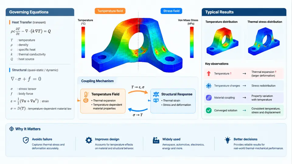
Thermal-structural coupling is the class of multiphysics problems in which a temperature field and a structural deformation field influence each other. In finite element analysis (FEA), this interaction is not a single equation but a coupled system: the thermal solution produces a temperature distribution, that distribution drives thermal strain, and the resulting deformation and stress state may in turn alter the thermal boundary conditions or material response. Understanding this loop is the foundation for every subsequent chapter in this course.

1.1 The Two Governing Fields

The thermal side is governed by the transient heat conduction equation. In its strong form, for a domain with density ρ, specific heat capacity c_p, and conductivity tensor k:

ρ c_p ∂T/∂t = ∇ · (k ∇T) + Q

Here T is temperature, t is time, and Q is volumetric heat generation. The structural side is governed by the momentum balance (quasi-static form is sufficient for most thermal-structural problems):

∇ · σ + f = 0

where σ is the Cauchy stress tensor and f represents body forces. The bridge between the two fields is the constitutive relation for thermoelasticity:

σ = C : (ε − ε_th),   ε_th = α (T − T_ref) I

In this expression, C is the fourth-order elasticity tensor, ε is the total strain, ε_th is the thermal strain, α is the coefficient of thermal expansion (CTE), T_ref is the stress-free reference temperature, and I is the identity tensor. The term (T − T_ref) is critical: if T_ref is set incorrectly, the entire stress field is offset by a constant, a common source of unrealistic results.

1.2 Coupling Mechanisms: One-Way vs. Two-Way

Coupling strength determines which solution strategy is appropriate. In one-way coupling, the thermal field affects the structure but not vice versa. This is valid when deformations are small enough that they do not change heat transfer paths, contact areas, or material properties. The workflow is sequential: solve thermal, map temperatures to the structural mesh, solve structural. Most electronic packaging, engine component, and heat-exchanger analyses fall into this category.

In two-way coupling, the structural response feeds back into the thermal problem. Typical feedback paths include:

• Contact conductance: as surfaces deform, the real contact area and gap thickness change, altering thermal contact resistance.
• Large deformation: geometry changes modify conduction paths and radiation view factors.
• Temperature-dependent properties: CTE, conductivity, and yield strength vary with temperature, so the structural solution changes the thermal material state.
• Frictional heating: relative sliding generates heat that changes the temperature field.

Two-way coupling requires iteration between the thermal and structural solvers within each time step or load step. The convergence criterion is typically a norm on the change in temperature and displacement between iterations.

1.3 Industrial Relevance

Thermal-structural coupling appears across nearly every advanced manufacturing sector. In aerospace, turbine blades experience temperature gradients exceeding 500 °C across a few millimeters, producing thermal stresses that can exceed mechanical loads. In electronics, solder joint fatigue under power cycling is driven by CTE mismatch between silicon, copper, and PCB laminate. In automotive, exhaust manifolds and brake discs undergo severe thermal cycling that governs low-cycle fatigue life. In energy, nuclear reactor components and solar receivers must maintain structural integrity under high heat flux.

The industrial value of coupled FEA is that it replaces expensive thermal cycling tests with predictive simulation, allowing designers to evaluate material choices, cooling strategies, and geometry changes before hardware exists. However, the accuracy of these predictions depends entirely on correct governing equations, consistent reference temperatures, and appropriate coupling assumptions.

1.4 A Minimal Worked Example: Clamped Bar Under Thermal Load

Consider a steel bar of length L = 200 mm, cross-section 20 mm × 20 mm, fully clamped at both ends. The reference temperature is T_ref = 20 °C. The bar is heated uniformly to T = 120 °C. Material: E = 210 GPa, α = 12 × 10⁻⁶ /°C, ν = 0.3.

Because the bar is fully constrained, total strain ε = 0. The thermal strain is ε_th = α(T − T_ref) = 12 × 10⁻⁶ × 100 = 1.2 × 10⁻³. The mechanical strain is therefore ε_mech = ε − ε_th = −1.2 × 10⁻³. The axial stress is σ = E ε_mech = 210 × 10⁹ × (−1.2 × 10⁻³) = −252 MPa (compressive).

In a one-way FEA workflow, you would: (1) assign thermal boundary conditions — here, a uniform temperature of 120 °C on all nodes; (2) solve the steady-state thermal problem; (3) map the temperature field to the structural mesh; (4) apply fixed supports at both ends; (5) solve the static structural problem. The expected output is a uniform compressive stress of approximately 252 MPa. If your result differs significantly, check T_ref, unit consistency, and whether the thermal expansion was applied as an initial condition or as a load.

1.5 Common Pitfalls and How to Avoid Them

Reference temperature mismatch. If the thermal solver uses 0 °C as the stress-free reference but the structural solver uses 20 °C, the stress will be offset by E α × 20. Always define T_ref once and propagate it consistently.

Ignoring temperature-dependent properties. For large temperature swings (e.g., 20 °C to 800 °C), constant CTE and yield strength introduce errors of 20–50%. Use tabulated property data and enable temperature interpolation.

Incorrect contact definition. In thermal-structural contact, you must define both mechanical contact (normal and tangential behavior) and thermal contact conductance. A common error is to define only mechanical contact, which creates an adiabatic gap and produces unrealistic temperature jumps.

Mesh mismatch between domains. If the thermal and structural meshes differ, the mapping algorithm introduces interpolation error. For strong gradients, use a consistent mesh or a conservative mapping scheme.

1.6 What This Chapter Establishes

This chapter has defined the two governing equations, the thermoelastic constitutive bridge, the distinction between one-way and two-way coupling, and the industrial contexts where each applies. It has also demonstrated a closed-form verification case and identified the most frequent modeling errors. These elements form the reference frame for the remainder of the course: every subsequent technique — whether transient thermal loading, contact conductance calibration, or fatigue post-processing — builds on the equations and coupling logic introduced here.