1. Course overview
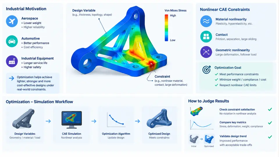
Structural optimization has matured to the point where linear static responses are no longer the bottleneck. The real difficulty begins when the design must satisfy constraints that only appear after the structure has yielded, buckled, contacted another body, or accumulated damage. In these regimes, the relationship between a design variable and a constraint is nonlinear, path-dependent, and frequently non-smooth. This chapter establishes the vocabulary, the industrial motivation, and the end-to-end workflow that the remaining 29 chapters build upon.
What "Nonlinear CAE Constraints" Actually Means
A structural optimization problem is conventionally written as: minimize an objective f(x) subject to constraint functions g_i(x) ≤ 0, where x is the vector of design variables. In linear optimization, g_i is typically a displacement, a stress, or a mass evaluated from a single linear solve. In nonlinear CAE, each evaluation of g_i requires an incremental Newton–Raphson solution over a load history, and the constraint may be any of the following:
- Geometric nonlinearity — large rotation or large strain, where the stiffness matrix depends on the current configuration. Constraint examples: tip deflection under a follower load, snap-through limit load.
- Material nonlinearity — plasticity, hyperelasticity, creep, or damage. Constraint examples: equivalent plastic strain
PEEQbelow an allowable, fatigue life above a target, residual stiffness after unloading. - Contact and boundary nonlinearity — changing contact status, friction, or self-contact. Constraint examples: contact pressure below a threshold, no penetration beyond a tolerance, reaction force within a range.
- Instability constraints — eigenvalue-based buckling or post-buckling reserve. Constraint examples: first linear buckling factor
λ₁ ≥ 1.5, or a nonlinear limit-load factor.
The defining property is that g_i(x) is not available in closed form. It is the output of a numerical solver, and its gradient with respect to x must be obtained either by finite differences, by the direct or adjoint method applied to the nonlinear equilibrium, or by a surrogate. This is what separates nonlinear-constrained optimization from classical sizing or topology optimization on linear models.
Why Industry Cares
Three industrial pressures make this topic unavoidable. First, lightweighting: automotive and aerospace structures are pushed to the point where linear analysis over-predicts capacity, so designs validated only linearly either fail in service or are over-conservative. Second, certification: crash, impact, and fatigue load cases are inherently nonlinear, and regulators require demonstration against them, not against linear surrogates. Third, cost of iteration: a single nonlinear load case can take minutes to hours, so an optimization loop that naively calls the solver thousands of times is economically impossible. The engineering response is a disciplined workflow that minimizes the number of nonlinear solves while still producing a certifiable design.
The Optimization–Simulation Workflow
The workflow below is the backbone of this course. It is a loop, not a pipeline, and the exit condition is a design that satisfies all nonlinear constraints with a margin, not merely a converged optimizer.
Each block in the diagram corresponds to a decision that materially affects both accuracy and runtime. The design variables x may be sizing parameters (shell thickness), shape parameters (control-point coordinates), or topology variables (element densities). The parametric model must regenerate cleanly for every x; a mesh that fails on an intermediate design will terminate the loop. The nonlinear solver returns not only the response but also a convergence status — a diverged increment is a failed constraint evaluation, not a valid g_i.
A Concrete Illustrative Example
Consider a simplified automotive lower control arm modeled with shell elements and an elastic–plastic material (E = 210 GPa, ν = 0.3, yield σ_y = 355 MPa, isotropic hardening). The design variables are three sheet thicknesses: t₁ (main body), t₂ (bushing boss), t₃ (ball-joint region), each bounded between 1.5 mm and 4.0 mm. The objective is mass. The nonlinear constraints are:
g₁: maximum equivalent plastic strainPEEQ_max ≤ 0.05under a 3 g vertical + 2 g lateral load history.g₂: first buckling factorλ₁ ≥ 1.8under a compressive load case.g₃: peak contact pressure at the bushing interface≤ 120 MPa.
A single evaluation of (g₁, g₂, g₃) requires one nonlinear static solve with roughly 20 load increments plus one eigenvalue extraction. On a typical workstation this is on the order of 4–8 minutes. A gradient by central finite differences with three variables costs six additional solves, i.e. ~30–50 minutes per design iteration. This arithmetic is why the course devotes later chapters to adjoint sensitivity and to surrogate-assisted constraint evaluation: without them, a 30-iteration optimization would consume days.
N_solves ≈ N_iter × (1 + N_grad) and multiply by the measured single-solve time. If the product exceeds your budget, reduce the problem — fewer variables, a coarser but verified model, or a surrogate — before touching the optimizer settings.
What This Course Delivers
The remaining chapters follow the loop in the diagram. Early chapters cover parametric modeling discipline and nonlinear solver settings that keep constraint evaluations reliable. The middle block addresses sensitivity analysis, constraint aggregation (e.g. Kreisselmeier–Steinhauser or p-norm for many local stress constraints), and surrogate construction for contact and buckling. Later chapters treat multi-objective trade-offs, robustness under scatter, and verification of the optimized design against the original nonlinear load cases. Throughout, the standard is reproducible engineering: given the same inputs, a reader should be able to reproduce the constraint values and the design decisions.
With this shared map in place — variables, parametric model, nonlinear solver, constraint extraction, sensitivity, optimizer, and convergence check — the next chapters can go deep on each block without losing the connection to the whole. The measure of success is not a converged optimizer log; it is a design that a nonlinear CAE engineer can defend against the original load cases with quantified margin.