1. Course overview
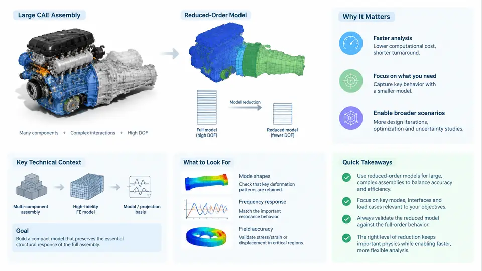
Large CAE assemblies are among the most demanding artifacts in modern virtual product development. A single full-vehicle crash model, an aircraft wing–fuselage build, or a wind-turbine drivetrain can easily contain 20–80 million degrees of freedom (DOF), tens of thousands of contact definitions, and hundreds of material laws. Running such a model once is expensive; running it inside a design-of-experiments loop, a multidisciplinary optimization, or a hardware-in-the-loop (HIL) test bench is often impossible. Reduced-order modeling (ROM) is the engineering discipline that makes those repeated evaluations tractable by replacing the high-fidelity model with a compact surrogate that preserves the response behavior of interest within a stated accuracy envelope.
This course treats ROM not as a single technique but as a workflow that spans model preparation, basis construction, operator evaluation, and validation. The scope is deliberately restricted to structural assemblies — stiffness, mass, damping, contact, and geometric nonlinearity — rather than thermal or CFD surrogates, although many of the mathematical tools overlap.
Why assemblies, not single components
Component-level ROM is a mature topic: a bracket, a beam, or a panel can be reduced with a few dozen modes and validated against a modal test. Assemblies introduce three complications that dominate the engineering effort:
- Interface coupling. Substructures exchange forces and displacements through bolted flanges, welds, bushings, and splines. A ROM that is accurate in isolation can produce large errors once connected, because the interface stiffness and the local mode shapes at the boundary are exactly what the reduction tends to truncate.
- Contact and nonlinearity. Hundreds of contact pairs, gaps, and preloaded joints mean the effective stiffness changes with load path. Linear modal reduction alone cannot represent this; the ROM must carry parameter dependence.
- Scale disparity. A 5 mm mesh in a weld toe coexists with a 500 mm mesh in a floor pan. Uniform reduction wastes DOF on regions that never participate in the response of interest.
The practical consequence is that assembly ROM is as much a partitioning and interface problem as it is a linear-algebra problem. The course therefore spends significant time on how to decide what to reduce, what to keep full, and how to certify the coupled result.
The technical context: where ROM sits in the CAE stack
It helps to place ROM relative to the tools engineers already use. A full-order model (FOM) is the reference: the assembled mesh, solver deck, and boundary conditions that define the truth for a given load case. A ROM is a projection of that FOM onto a low-dimensional subspace, plus a strategy for evaluating the projected operators efficiently. The figure below shows the data and decision flow from an assembled CAE model to a validated ROM and its downstream consumers.
What "reduced order" actually means in practice
A ROM is defined by a projection matrix Φ ∈ R^(N×r) with r ≪ N, and a reduced state q ∈ R^r such that the physical displacement is approximated by u ≈ Φ q. Substituting into the assembled equation of motion and pre-multiplying by Φᵀ gives the reduced system:
M̂ q̈ + Ĉ q̇ + K̂ q = f̂(t)
where  M̂ = Φᵀ M Φ,  Ĉ = Φᵀ C Φ,  K̂ = Φᵀ K Φ,  f̂ = Φᵀ f
The engineering question is never "can we project?" — it is "which Φ keeps the response error inside tolerance for every load case we care about?" For assemblies, the most widely used answer is the Craig–Bampton basis: fixed-interface normal modes for the interior, plus constraint modes for every interface DOF. If an assembly has 4,000 interface DOF and we keep 60 interior modes per substructure, a 6-million-DOF model can collapse to roughly 5,000–8,000 reduced DOF while retaining interface fidelity.
Motivation: the economics of repeated evaluation
Consider a representative example. A full-vehicle frontal-crash FOM with 35 million DOF takes about 9 hours on 64 cores. A design study with 200 variants would consume roughly 1,800 core-hours per load case. If a Craig–Bampton ROM with 6,000 DOF reproduces the intrusion and peak-acceleration metrics within 5%, the same study runs in minutes per variant on a workstation. The ROM build itself — one modal solve plus interface reduction — costs a few hours once. The break-even point is typically reached after 5–15 design evaluations, which almost every realistic program exceeds.
The motivation is not only speed. A ROM enables interactive and embedded use: a 1 ms cycle time for HIL, a differentiable operator for gradient-based optimization, and a compact artifact that can be shipped to a supplier without exposing the full mesh. These are qualitatively different capabilities, not just faster versions of the same simulation.
Scope boundaries and what this course does not cover
To keep the material actionable, the course draws explicit boundaries:
| In scope | Out of scope |
|---|---|
| Linear and mildly nonlinear structural assemblies | Large-strain metal forming, fluid–structure interaction |
| Craig–Bampton, POD, and modal derivatives | Deep-learning surrogates as a primary method |
| Interface reduction and coupling strategies | Acoustic or thermal ROM |
| Error metrics and acceptance criteria | Solver-internal parallelization |
| Parametric and real-time ROM | Model updating from test data |
How the course is organized
The 30 chapters follow the natural build order of an assembly ROM project. Early chapters establish the mathematical foundation and the partitioning decisions. The middle block covers basis construction, interface treatment, and nonlinear extension. The later block addresses validation, parametric ROM, real-time deployment, and a full worked case study on a bolted automotive subframe. Each chapter includes a reproducible example with concrete parameters, expected observable outputs, and typical failure symptoms so that you can diagnose your own models rather than only follow a recipe.
By the end of this course you should be able to look at a large CAE assembly, decide which regions to reduce and which to retain, construct a Craig–Bampton or POD basis with defensible mode counts, assemble and solve the reduced operator, and certify the result against the full-order reference with quantitative error metrics. The next chapters begin with the mathematical foundations of projection-based reduction.