📚 Course ContentsChapter 1 Course overview

1. Course overview

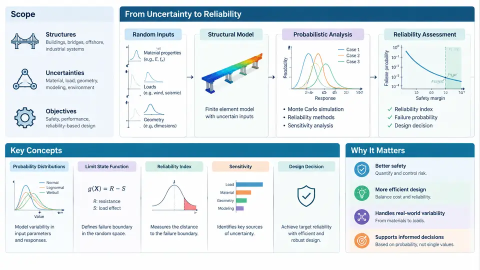
Deterministic finite element analysis answers a narrow question: given one fixed set of dimensions, material properties, and loads, what is the structural response? Real hardware never behaves that way. A batch of 500 stamped brackets has wall thicknesses scattered around the nominal value, yield strengths that vary from heat to heat, and service loads that depend on operator behavior and duty cycle. Probabilistic structural simulation exists to answer the question deterministic analysis cannot: what is the probability that the structure violates a performance requirement, and which uncertain inputs dominate that probability?

This course builds the full technical chain from uncertainty characterization through surrogate-accelerated simulation to reliability-based design decisions. This opening chapter defines the vocabulary, the scope boundaries, and the engineering context that the remaining 29 chapters will develop in depth.

What "Probabilistic" Changes About the Analysis

In a deterministic workflow, every input is a scalar. In a probabilistic workflow, each uncertain input is a random variable with a distribution type, parameters, and — critically — a correlation structure with other variables. The structural model itself (mesh, element formulation, boundary conditions) does not change; what changes is that it is evaluated many times, and the outputs are treated as random variables too.

The formal object of study is the limit state function g(X), where X = (X₁, X₂, …, Xₙ) is the vector of random inputs. The convention used throughout this course is:

g(X) > 0 → safe region (resistance exceeds demand)
g(X) = 0 → limit state surface
g(X) < 0 → failure region

The probability of failure is the integral of the joint probability density over the failure region:

P_f = P[g(X) < 0] = ∫_{g(X)<0} f_X(x) dx

Reliability index (first-order):   β = -Φ⁻¹(P_f)
For a linear g with normal X:      β = μ_g / σ_g

Two numbers therefore summarize structural safety: P_f (or equivalently β) and the sensitivity of P_f to each input. A design is not "reliable" in the abstract — it is reliable with respect to a stated set of limit states, distributions, and target probability. Changing any of those changes the answer, which is why documentation of assumptions is a first-class deliverable in this field, not an afterthought.

Where the Uncertainty Comes From

Uncertainty in structural simulation is conventionally partitioned into three categories, and the partition matters because each category is treated differently.

Category	Source	Typical treatment
Physical / aleatory	Inherent variability: material microstructure, manufacturing tolerance, load environment	Random variables with fitted distributions; irreducible by more testing
Model / epistemic	Simplified constitutive laws, mesh discretization, ideal boundary conditions	Model-form error factors, calibration against test data, Bayesian updating
Statistical	Finite sample size in the data used to fit distributions	Confidence intervals on distribution parameters; widened design margins

A common beginner error is to assign a normal distribution to every input by default. Thickness and strength are typically better described by lognormal or Weibull distributions because they are strictly positive and right-skewed. Load extremes are often modeled with Gumbel or generalized extreme value distributions. The choice of distribution tail directly controls P_f when the target probability is small, so distribution selection is an engineering decision with safety consequences.

The Computational Problem

The naive approach — Monte Carlo simulation — draws N samples from f_X(x), runs the FE model N times, and counts the fraction with g(X) < 0. It is robust and embarrassingly parallel, but the sample size required for a small probability is brutal:

Required N ≈ 10 / P_f   (for ~10% coefficient of variation on the estimate)

Target P_f = 1e-3  →  N ≈ 10,000 FE runs
Target P_f = 1e-6  →  N ≈ 10,000,000 FE runs

When a single nonlinear implicit FE solve takes 20 minutes, ten million runs is not a plan. This is the central tension of the field, and it drives the entire methodological toolkit covered in this course: first-order and second-order reliability methods (FORM/SORM) that linearize the limit state in a transformed standard normal space; importance sampling and subset simulation that concentrate samples near the failure domain; and surrogate models — polynomial chaos expansion, Kriging/Gaussian process, and neural network surrogates — that replace the FE solver with a cheap approximation trained on a few hundred well-chosen runs.

Key framing: Every advanced method in this course is a trade between three quantities — number of expensive model evaluations, accuracy of the P_f estimate, and robustness when the limit state is highly nonlinear or the input dimension is large. No method wins on all three. Selecting the right one for a given problem is the core engineering skill being taught.

How the Pieces Fit Together

The workflow below shows the technical context of the course. Uncertainty quantification feeds the simulation engine, which feeds the reliability and sensitivity analysis, which feeds the design decision. The feedback loop is essential: sensitivity results tell you which variables to characterize more precisely, and design changes alter the limit state surface, requiring re-analysis.

Scope Boundaries and What This Course Does Not Cover

To keep the technical focus sharp, the course treats the following as given inputs rather than topics of study: the underlying deterministic FE formulation (assumed known), the physics of the specific failure modes (assumed to be identified by conventional analysis), and the regulatory framework that sets target reliability levels (referenced but not derived). What the course does cover in depth is the probabilistic layer: how to build defensible input distributions from limited data, how to choose and validate a simulation strategy, how to interpret and communicate the resulting probabilities, and how to close the loop into design.

Reading the reliability index: β = 1.0 corresponds to P_f ≈ 1.6×10⁻¹; β = 3.0 to P_f ≈ 1.3×10⁻³; β = 4.0 to P_f ≈ 3.2×10⁻⁵. Civil and aerospace targets commonly sit between β = 3.0 and β = 4.5 depending on consequence class. Note that these mappings assume a normal distribution for g; for strongly non-normal cases the mapping is approximate and should be verified by simulation.

What You Will Be Able to Do

By the end of the course, you should be able to take a real component with scattered inputs, build a defensible probabilistic model, select an appropriate reliability method based on the target P_f and available compute budget, run the analysis, validate the result against a reference where possible, and translate the output into a design decision with an explicit statement of confidence. The chapters that follow develop each link in that chain — starting with the mathematical foundations of random variables and limit states, then moving through sampling, surrogate construction, reliability algorithms, sensitivity analysis, and reliability-based design optimization.

The single most important habit to build from this chapter onward: never report a probability of failure without stating the distributions, the limit state definition, the method used, and the verification performed. A number without that context is not a reliability result — it is a guess with decimal places.