1. Nonlinear FEA for complex structures

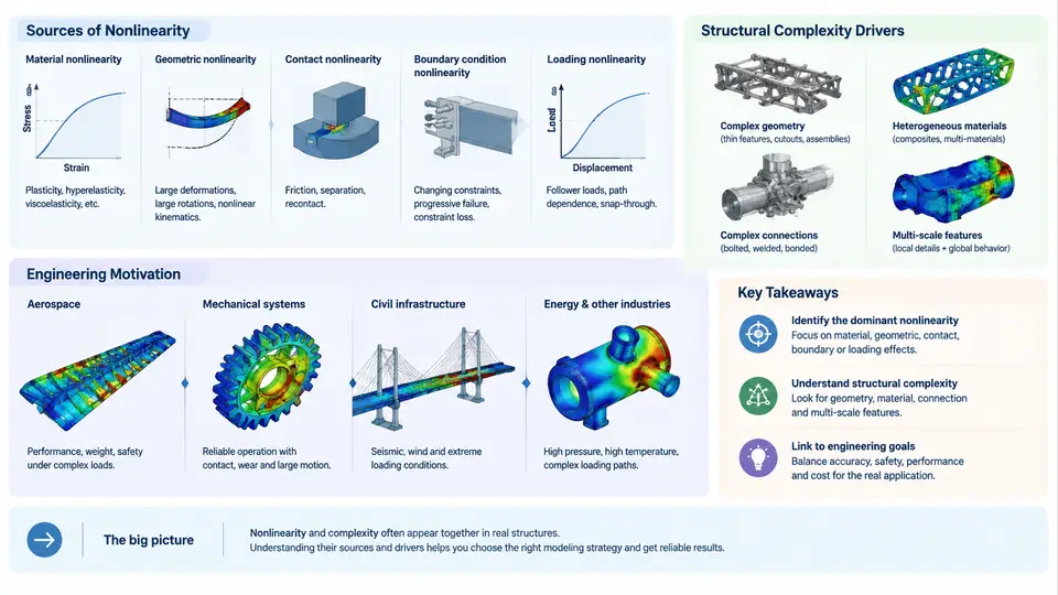
Linear static finite element analysis rests on three quiet assumptions: stiffness is constant, displacements are infinitesimal, and boundary conditions never change. For a stiffened panel under moderate load, those assumptions are excellent. For a thin-walled launch-vehicle shell buckling under compression, a rubber engine mount at 40% strain, or a bolted flange joint that separates and re-contacts during a pressure cycle, they are simply wrong. Nonlinear FEA exists because the physics of real structures violates all three assumptions simultaneously, and the errors from ignoring that violation are not small perturbations — they are order-of-magnitude errors in predicted load capacity, failure mode, and fatigue life.

Where Nonlinearity Actually Comes From

Three distinct mechanisms produce nonlinear force–displacement behavior, and they must be diagnosed separately because each demands different solver settings, different element formulations, and different verification strategies.

Geometric nonlinearity arises when changes in configuration alter the load path. The governing equilibrium is no longer K·u = F with constant K; it becomes K(u)·u = F, where the stiffness matrix itself depends on displacement. Two effects dominate. First, large rotations redistribute internal forces: a cantilever tip deflection of 15% of its length already produces membrane stiffening that linear analysis misses entirely. Second, instability phenomena — buckling and post-buckling — are purely geometric. A cylindrical shell with radius-to-thickness ratio R/t = 500 may exhibit a linear eigenvalue buckling load of 1.0 MPa but a nonlinear collapse load of only 0.35 MPa due to imperfection sensitivity. Linear analysis cannot capture this knockdown at all.

Material nonlinearity appears whenever stress and strain are not proportional. Metal plasticity beyond yield, hyperelastic rubber, viscoelastic polymers, and concrete cracking all fall here. The critical distinction is path dependence: plastic strain accumulates irreversibly, so the solution depends on load history, not just the final load level. A pressure vessel cycled to 90% of yield and back will retain residual stresses that a monotonic analysis never predicts.

Contact and boundary nonlinearity is the third source and often the most computationally punishing. Contact conditions are inequality constraints: a gap either opens or closes, and the active constraint set changes as the solution evolves. Each change is a discontinuity in the stiffness matrix. A bolted joint with 12 bolts may require hundreds of contact iterations to converge, and a gear tooth pair in mesh involves sliding contact with friction, adding another layer of path dependence.

What Makes a Structure "Complex"

Complexity in this context is not a vague descriptor — it has specific, measurable drivers that determine mesh strategy, solver cost, and modeling risk.

Topological complexity means many interacting components with distinct load paths: a wing box with spars, ribs, stringers, and skin; a satellite bus with honeycomb panels, inserts, and bracket interfaces. Each interface is a potential contact region and a potential stress concentration.

Material heterogeneity means the structure contains materials with orders-of-magnitude different stiffness — steel inserts in composite laminates, for example, where E_steel ≈ 210 GPa and E_carbon_epoxy ≈ 70 GPa in fiber direction but only 10 GPa transverse. This mismatch creates ill-conditioned stiffness matrices and slow convergence.

Scale span is the ratio between the largest and smallest features that must be resolved. A full aircraft fuselage section may span 6 m while a fastener hole is 6 mm — a 1000:1 ratio. Resolving both in one mesh is impractical; submodeling or global-local techniques become mandatory.

Non-proportional loading and load-path interaction add another dimension. A structure under simultaneous internal pressure, axial compression, and thermal gradient does not simply superpose responses. The pressure may stabilize a shell against buckling while the thermal gradient softens it — the interaction is nonlinear and must be analyzed as such.

Why This Matters in Practice: A Worked Example

Consider a representative aerospace bracket assembly: a titanium fitting (Ti-6Al-4V, E = 114 GPa, σ_y = 880 MPa) bolted to a carbon-fiber composite panel (E₁ = 135 GPa, E₂ = 10 GPa, G₁₂ = 5 GPa) through four M8 bolts, loaded by a 12 kN transverse force at a 150 mm offset. This is a deliberately modest example — one bracket, four fasteners — yet it already exhibits all three nonlinearity sources.

Geometric: The 150 mm moment arm produces a tip rotation that, at full load, exceeds 8°. Linear analysis underestimates the bending stress at the fitting root by approximately 12–18% because it neglects the P-δ moment amplification from the axial load component.

Material: The titanium fitting yields locally at the bolt-hole bearing surface. A linear analysis reports a stress of 1,050 MPa — above yield — but cannot tell you whether the plastic zone is contained or spreads to cause net-section failure. Only an elastic-plastic analysis with a proper hardening curve can answer that.

Contact: The bolted joint is not rigid. Under load, the composite panel and titanium fitting separate on the tension side of the joint, transferring load through bearing at the holes rather than through friction. The joint stiffness drops by roughly 40% once separation begins. A linear model with bonded contact completely misses this stiffness transition and predicts a load path that does not exist.

What Nonlinear FEA Delivers That Linear Cannot

The engineering value of nonlinear FEA is not merely "more accurate stress numbers." It changes what questions you can ask. Linear analysis answers: "What is the stress at this point under this load?" Nonlinear analysis answers: "At what load does the structure collapse? How does it fail? Does it snap through or fail gradually? What residual stresses remain after unloading? Does the joint stay sealed under pressure cycling?"

These are the questions that determine whether a design meets certification requirements, whether a fatigue life prediction is credible, and whether a weight-saving redesign is safe. The remainder of this course builds the practical skills to answer them: element selection for large deformation, material model calibration, contact definition and stabilization, solver convergence strategies, and verification against physical tests.

The starting point is always the same: identify which nonlinearity sources are active, quantify the structural complexity drivers, and choose a modeling strategy that captures the physics without exceeding available computational resources. That diagnostic step — performed before any mesh is generated — determines whether the analysis will be a useful engineering tool or an expensive source of false confidence.